There are two common measures of interest rate risk, i.e. duration and convexity. These are discussed in detail here.

1.1.         Duration

a.  The duration measures the sensitivity of a bond’s full price to the changes in the bond’s own yield or, more generally, changes in the benchmark rate.

b.  In the calculation of duration, it is assumed that all the other variables are held constant.

c.  Consider the following diagram: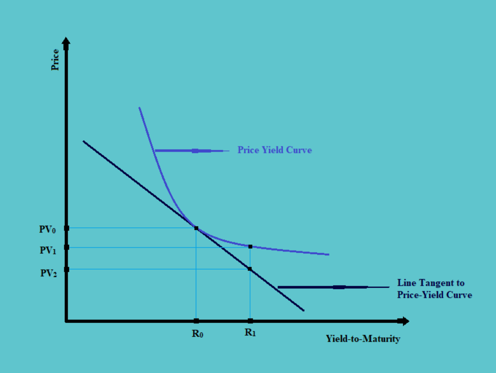

In the above figure, we have a rate of interest are there on the x-axis, and the price of the bond is there on the y-axis. We can see that, when there is an increase in the interest rates, there is a decrease in the present value of the bond or its price. On considering the price-yield curve, the decrease in price should be till the point PV₁. However, the price cannot exceed the line tangent to the price yield Thus, the price would fall to the point PV₂. This is called the convexity adjustment.

As the changes in the rate of interest keep increasing, the difference in the change of price also increases.

The linear line tangent to the price-yield curve depicts the duration of the bond. This duration represents the approximate amount of time a bond would have to be held for the market discount rate to be realized.

d.  For example, if there is a 10-year, 8% bond paying coupons annually, with a YTM of 10.4% as in the above example. If there is an increase in the YTM, there will be an increase in the income from the reinvestment of the coupons and a capital loss on the sale of the bonds.

If the bonds are held for 7.0029 years, the sum of the gains from reinvestment of the coupons and the capital loss on the sale of the bonds equals zero. Thus, the duration of the bonds is 7.0029 years.

1.1.1.     Types of Duration

a.  There are two important types of durations, i.e. the yield duration and the curve duration.

b.  The yield duration is the measure of the sensitivity of the price of the bond to its own YTM. There are different types of yield duration such as Macaulay’s Duration, Modified Duration, Money Duration, Price Value of a Basis Point (PVBP).

c.  The curve duration is the measure of the sensitivity of the price of the bond to the benchmark yield. The examples of curve duration are Government Yield Curve, Spot Curve, Forward Curve, Par Curve. The Par Curve is the most often used measure of curve duration.

The curve duration bond is mainly used with complex bonds and also with financial assets or liabilities that have interest rate risk but are not bonds

1.1.2.     Macaulay’s Duration

a.  The Macaulay duration is the weighted average term to maturity of the cash flows from a bond.

b.  It can be calculated using the following formula:

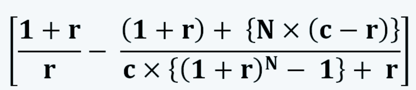
c.  It can also be calculated using the following closed formula, instead of the above complex formula:

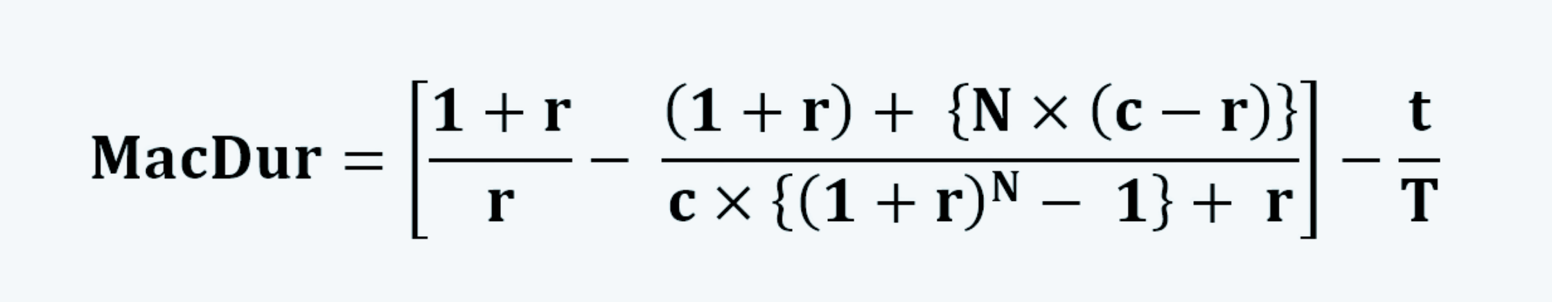Where c is the coupon payments.

d.  We can explain the calculation of Macaulay’s duration with the help of the previous example of a 10-year, 8% annual bond, having a YTM of 10.4%:

The duration of the bond here is 7.0029

1.1.3.     Modified Duration

a.  The modified duration is a modification of Macaulay’s Duration.

b.  It can be calculated by dividing Macaulay’s Duration by (1+r).

c.  In the above example, the modified duration of the bond is:

ModDur = 7.0029 / (1+0.104) = 6.3432

d.  The modified duration provides a linear estimate of the percentage price change for a bond, given a change in its YTM. Therefore,

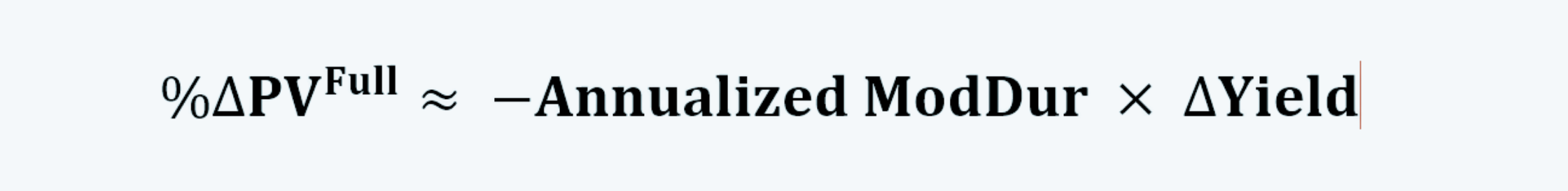e.  Thus, in the above example, if there is a 100 bps increase in the YTM to 11.4%, the total change in the full present value would be:

%∆PV^Full ≈ -6.3432 × 0.0100 = -6.3432%

However, if there is a 100 bps fall in the YTM to 9.4%, the total change the full present value would be:

%∆PV^Full ≈ -6.3432 × -0.0100 = 6.3432%

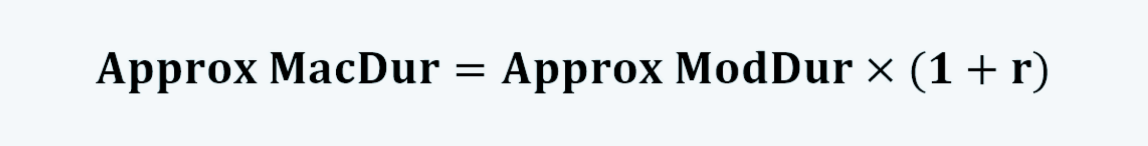
f.  If we know the value of Macaulay’s duration, we can calculate the modified duration by simply dividing the same with (1+r). However, if Macaulay’s duration is not known, we can approximate the value of modified duration using the following formula:

g.  For the smaller changes in the yield, the approximate modified duration equals the annualized modified duration. Therefore, for the smaller changes in yield:

h.  In the above example of a 10-year, 8% annual bond, having a YTM of 10.40 %, the present value of the cash flows of the bond is $ 85.503075. If there are a 25 bps increase and a decrease in the YTM of the bond, its PV would be $ 84.1618 and $ 86.8739. The approx modified duration of the bond would be:

Approx. ModDur = (86.8739 – 84.1618) / (2 × 0.0025 × 85.503075) = 6.34377

1.1.4.     Effective Duration

a.  Effective duration is used to calculate the approximate and modified duration for the complex bonds with embedded options.

b.  It can be calculated using the following formula:

c.  We can explain the concept of effective duration with the help of the following figure:

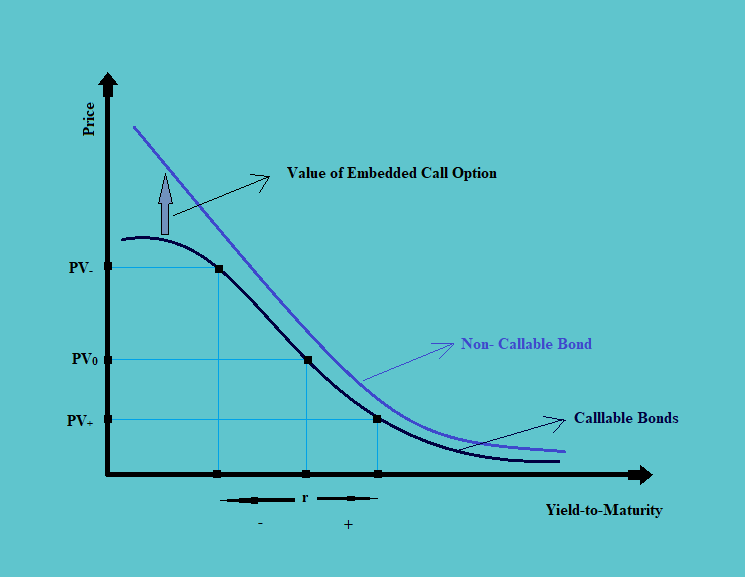
In the above figure, the value of the bond is reflected through the curved lines. When there is a fall in the yield, the gap between the callable and the non-callable bonds increases. This is mainly because, when there is a fall in the interest rates, it becomes more worthy for the issuer to call the bonds and issue the same at the lower rates. Thus, there is an increase in the value of embedded call options. But when there is an increase in the interest rates, the value of the call options becomes almost nil. Therefore, there is generally no gap between the price of a callable and non-callable bond.

There is, thus, a need to find the value of the call option in case of the fall in interest rates, and this requires an option pricing model for valuing the PV_–.

d.  The interest rates are made up of two components, i.e. credit spread and benchmark yield. The callable bonds may be called if there is either a decrease in the credit spread or the benchmark yield. For a decrease in the credit spread, there will be a change in the credit duration, which can be calculated to find the effective duration. On the other hand, for a decrease in the benchmark yield, there is a change in curve duration, which needs to be calculated.

e.  The effective duration can also be used for the floating rate notes (FRNs), mortgage-backed securities (MBSs), defined benefit pension plans (i.e. DBPP for the retirement obligations).

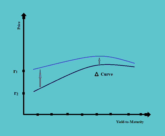
f.  The change in the curve (as calculated for the effective duration) is not always equal to the change in yield (as required for the calculation of modified duration).
The change in the curve is based on the par curve, whereas, the change in yield is based on the spot curve. When the par curve is shifted, there is also a shift in the spot curve; but the shift is not in a parallel fashion. Thus, the changes in both are not always equal.

The changes in yield and the curve are approximately equal in the following situation:

     i.  When the par curve is flatter,

    ii.  The shorter is the duration of the bond, and

   iii.  Closer is the price to the par.

1.1.5.     Key Rate Duration

a.  The effective duration assumes a parallel shift in the yield curve for the calculation of the change in portfolio value. However, if the yield curve shifts in a non-parallel fashion, a portfolio’s effective duration cannot be used to estimate the change in the portfolio value.

b.  For the calculation of effective duration, we have ‘2 × ∆Curve × PV₀’ in the denominator. The value of change in curve remains the same if there is a parallel shift in the yield curve, i.e. if the maturity of the bonds is the same. However, in a portfolio, there are bonds with different maturities. Thus, the shift in the yield curve may not always be parallel. This would result in different values of ‘∆Curve’.

c.  Key-rate duration is the duration at a specific maturity on a yield curve. Therefore, for a non-parallel shift in the yield curve, the key-rate duration must be used to estimate the change in portfolio value (i.e. ‘%∆Portfolio Value’).

d.  The key-rate duration is calculated for each maturity separately, using the following formula:

e.  So, if there are ‘n’ number of maturities, the effective duration can be calculated using the key-rate duration calculated for each maturity as follows:

f.  And, change in portfolio value can be calculated as follows:

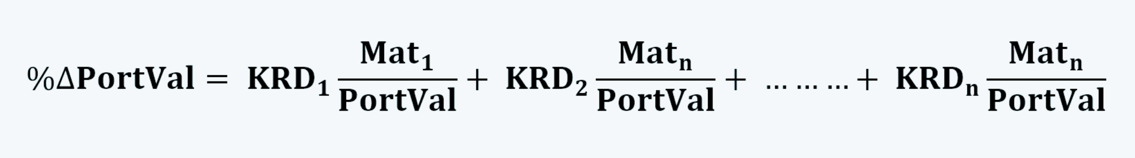Where KRD is the key-rate duration.

1.2.         Properties of Bond Duration

a.  As discussed, Macaulay’s duration can be calculated using the formula:

b.  Thus, Macaulay’s duration is a function of coupon payments, rate of interest, time to maturity, and a number of payments.

MacDur = ∫ (c, r, N, t)

c.  Thus, we can find the properties of bond duration by considering one of these as variables and others as constant.

d.  To begin with, let us consider time (t) as the variable and everything else as constant.

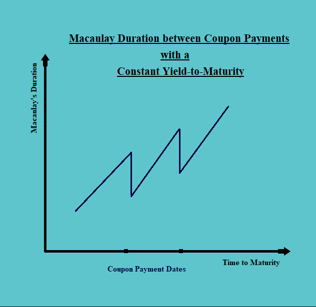
The Macaulay duration decreases smoothly as t goes from t = 0 to t = T, which creates a “saw-tooth” pattern. This is mainly because, as time progresses, the time up to maturity keeps decreasing. The duration of the bond also keeps decreasing till the maturity date. On the coupon date, the duration again increases, but not as much as the previous high, because the value of ‘N’ (i.e. the number of coupons) has reduced by one on that date.

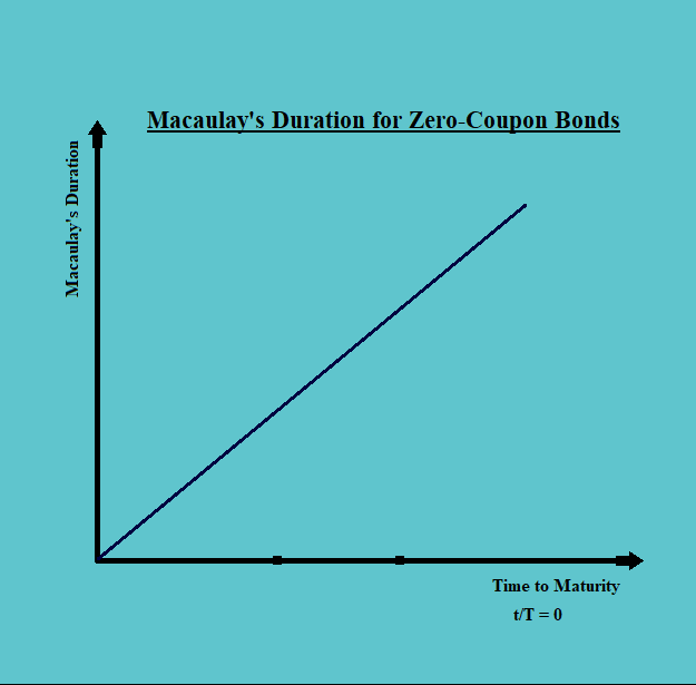
e.  For the zero-coupon bonds, the duration line is a straight line with a slope of 1 (i.e. an angle of 45^ͦ. This is mainly because the duration is only affected by the time and everything else does not have an impact.

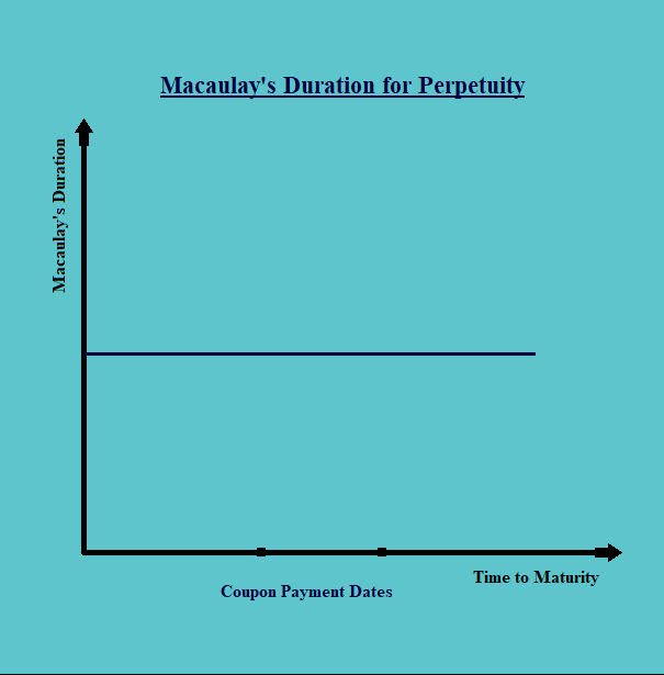
f.  For perpetuity, the N tends to infinity, thus the term,

also tends to 0, (because the denominator tends to infinity here). Thus, the duration line is a straight horizontal line with [(1+r) / r] as intercept.

     i.  For a premium bond, the duration curve is upward sloping, but always below the zero-coupon bond. This is mainly because a bond with the coupon will always have a weight for the coupon payments. The duration curve of a premium bond approaches the duration curve of the perpetuity as it approaches its maturity.

This is mainly because, for the premium bonds, the term ‘c-r’ is always positive. Hence the term 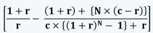is also positive. Thus, the equation of the whole line is [{(1+r)/r} – (a positive number)] which is also positive, and less than the term [(1+r) / r], which is the equation of perpetuity’s duration curve.

    ii.  Similarly, for a discount bond, the term ‘c-r’ may also get negative. Thus it may rise above the perpetuity demand curve but will tend towards the same as the bond approaches its maturity.

The duration curve of a discount bond is also a positively sloping curve, lying below the duration curve of a zero-coupon bond.

g.  The duration tends to increase, with an increase in the time to maturity of the bond.

h.  As we can see in the above figure, the bonds that carry higher coupons, have their demand curves below the ones that have lower coupons (it should be noted that the bonds issued at a premium, generally have to pay higher coupons in comparison to the bonds issued at par or discount). Thus, the bonds with higher coupons tend to have a lower duration.

i.  The bonds with lower YTM tend to have higher duration. This is mainly because the bonds with lower YTM have higher weights.