1.1. Marginal Returns and Productivity
a. Before we discuss the marginal returns and productivity, we first need to understand the production process.
i. The process of production requires certain factors of production or inputs. These include factors such as labor, capital, and others.
We would be primarily discussing labor and capital only. The units of labor and capital are denoted by ‘L’ and ‘K’ respectively. And, the cost of labor and capital are the wage rate (denoted by ‘w’) and interest rate (denoted by ‘r’).
ii. All the factors go into the production process to produce the output or product.
iii. The amount of production can be measured using any of the three measures, i.e. total product, average product, or marginal product.
The total product is the total quantity of goods produced during a period.
The average product is the average of the production, per unit of input. Thus, the average product can be calculated by dividing the total product by the number of units of labor if the labor is the prime unit of production.
The marginal product of a unit of a factor of production is a number of additional units of output produced, by using one more additional unit of a factor of production.
b. We can explain the concept of total, average and marginal products with the help of the following example:
|
Labor (L) |
Total Product (QL) |
Average Product (APL) |
Marginal Product (MPL) |
|
0 |
0 |
0 |
0 |
|
1 |
250 |
250 |
250 |
|
2 |
490 |
245 |
240 |
|
3 |
705 |
235 |
215 |
|
4 |
912 |
228 |
207 |
|
5 |
1065 |
213 |
153 |
|
6 |
1182 |
197 |
117 |
|
7 |
1218 |
174 |
36 |
|
8 |
1208 |
151 |
-10 |
|
9 |
1170 |
130 |
-38 |
|
10 |
1120 |
112 |
-50 |
The first column of the table shows the number of units of labor used in the production. The second column shows the total product, or the total quantity produced. The third column shows the average product; it is the total product divided by the units of labor used (i.e. item in column 2 divided by the respective item in column 1). The third column represents the marginal product; it is calculated by dividing the change in the total product (column 2) by the change in units of labor (column 1).
This table can be presented in the form of a graph as follows:
From the above figure, we can see that the marginal product is increasing up to the first unit of production; beyond which the marginal product of the labor attars falling. The marginal product ultimately becomes negative after seven units of labor are used.
1.2. Breakeven & Shutdown Analysis
To say it simply, the breakeven point is attained when the total revenue from sales equals the total cost of production. And, a company needs to shut down when it starts earning negative profits, or the profits are less than zero.
1.2.1. Economic Profit, Accounting Profit & Normal Profit
a. There are different types of profits and costs involved in the profitability analysis. Different types of profits that need to be discussed are economic profit, accounting profit, and normal profit.
b. The economic profit is the difference between the total revenue and total economic cost of the company.
| Economic Profit = Total Revenue – Total Economic Cost |
The total economic cost is the total cost of the company, including the opportunity cost.
c. The accounting profit is the difference between the total revenue and the total accounting cost of the entity.
| Accounting Profit = Total Revenue – Total Accounting Cost |
d. Accounting cost is the explicit cost of the company. It is the monetary value of the economic resources used in production. It does not include the opportunity cost of production.
e. The normal profit can be defined in one of the two ways:
i. It is equal to the accounting profit, when the economic profit equals zero, i.e. when the accounting profit equals the opportunity cost.
ii. In other cases, the normal profit equals the opportunity costs.
f. We can explain the concept of economic profit, accounting profit, and normal profit with the help of the following example:
Suppose a project requires an investment of $ 100 million and the opportunity cost of investment is 10%, i.e. $ 10 million. During the year, the project earns revenue of $ 200 million and its accounting cost was $ 190 million. Thus,
i. The accounting profit of the company was:
Accounting Profit = Total Revenue – Total Accounting Cost = 200-190 = $ 10 million.
ii. The economic profit of the company is:
- Economic Profit = Accounting Profit – Opportunity Cost = 10-10 = 0
iii. The normal profit could be either the accounting profit or the economic cost, both of which in this case is $ 10 million.
1.2.2. Marginal Revenue
a. Marginal revenue is the additional revenue earned from increasing the output by one unit per time period.
b. The formula for calculating the marginal revenue is:
|
Marginal Revenue = ∆TR / ∆Q Where, ∆TR = Change in Total Revenue ∆Q = Change in Quantity |
c. For example, a company increases its production from 100 units to 150 units, this results in an increase in the total revenue from $ 80,000 to $ 112,500. Thus, the marginal revenue of the company would be:
MR = (112,500 – 80,000) / (150 – 100) = $650
d. The curve joining the marginal revenues at a different level of quantities produced and sold is called the marginal revenue curve.
e. The marginal revenue curve can reflect different attributes in different markets.
f. In the perfect competition markets, the prices are fixed, no matter what is the quantity offered for sale. Thus, the marginal revenue in such a market equals the average revenue (which is a price), and both are represented by a straight horizontal line on the graph.
g. In an imperfect competition market, the marginal revenue curve is a downward sloping curve, as follows:
h. The other way to interpret the marginal revenue is as follows:
i. The change in total revenue of the firm equals the price times the change in quantity plus the quantity times the change in price, or:
∆TR = P∆Q + Q∆P
ii. Thus the equation Marginal Revenue = ∆TR / ∆Q can be written as:
Marginal Revenue = (P∆Q + Q∆P) / ∆Q
iii. Or:
Marginal revenue = P*(∆Q / ∆Q) + Q*(∆P / ∆Q)
iv. Thus,
Marginal revenue = P + Q*(∆P / ∆Q)
1.2.3. Marginal Cost
a. Marginal cost is the increase in the total cost resulting from an increase in the output by one unit per time period.
b. The marginal costs are different for different time periods.
c. In the short-run, all the costs are fixed except the labor cost. Thus, the short-run marginal cost equals the wage divided by the marginal product of labor.
| SMC = W/ MPL |
The marginal product of labor is the additional output generated by an extra unit of labor employed.
d. Long-run marginal cost, on the other hand, is the change in total cost due to a change in one more unit of output, when all the inputs or factors of production are variable.
1.2.4. Average Variable Cost
a. The average variable cost is the total variable cost used in production divided by the number of goods produced.
b. The average variable cost can also be calculated by dividing the wage rate by the average product of labor (i.e. total labor cost divided by the number of goods produced.
| AVC = TVC / Q = W / APL |
1.2.5. Fixed Cost
a. Fixed Costs are the costs that generally remain the same over a given range but move to another constant level when the production increases.
b. For example, a unit of a company is currently producing 1 million units of a certain product. For this level of production, the company requires a general supervisor, paying a salary of $ 4,000 a month. But if the company doubles its production, it will require another supervisor. Thus, the cost of the salary of the supervisor is fixed up to a level of production, i.e. 1 million units. For any production above this level up to 2 million units, the cost of one more supervisor would be required to be incurred.
c. The costs that are fixed up to a certain level are also called quasi-fixed costs.
d. As seen above, the normal profits are also sometimes interpreted as the opportunity cost. In such a sense, the normal profits are also a part of the fixed cost.
1.3. Total, Average, Marginal, Fixed & Variable Costs
a. In the most simplistic form, the total, variable, and total fixed cost can be presented in the form of a graph as follows:
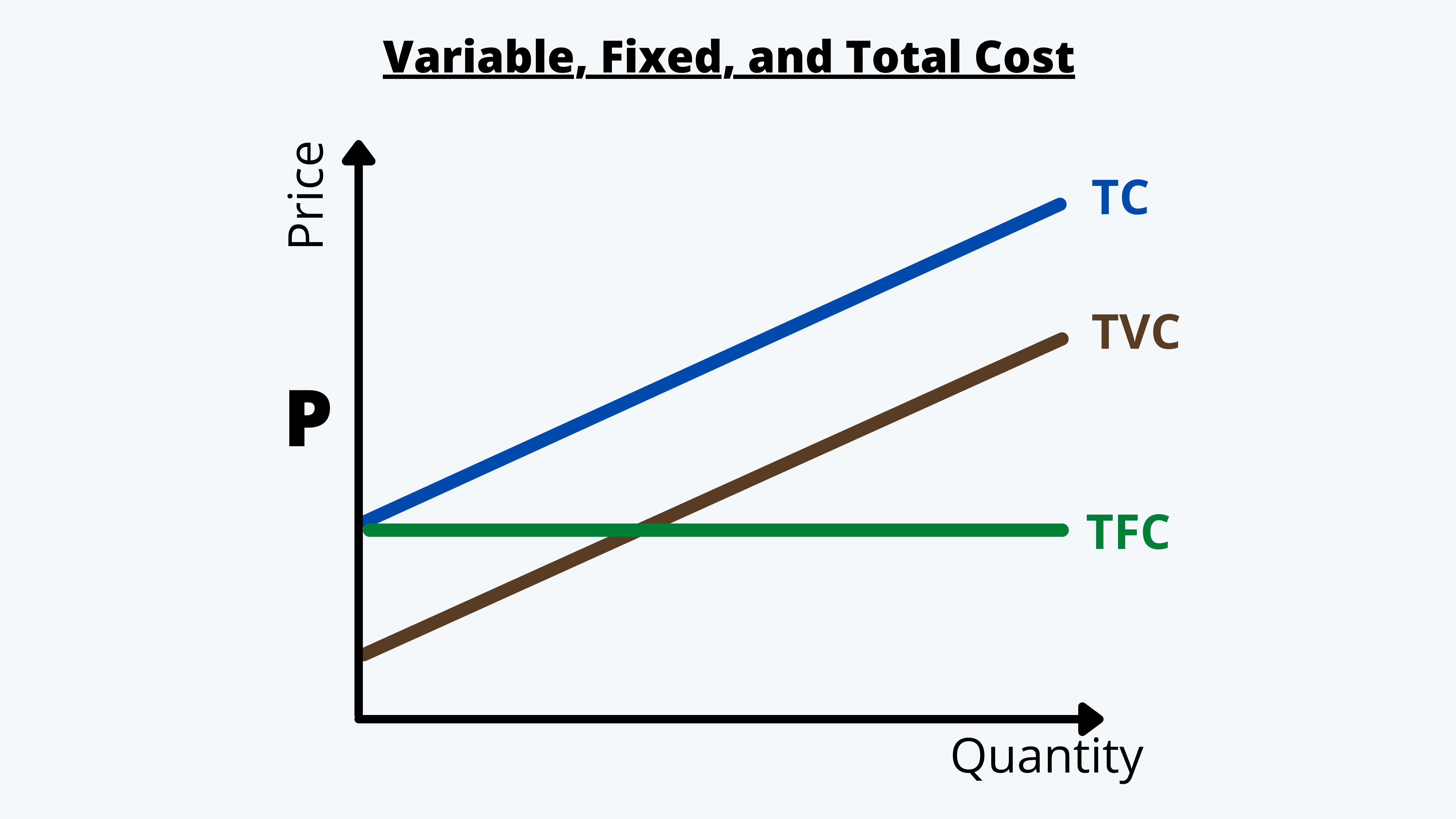
Here, the total cost is nothing but the total variable cost plus the total fixed cost.
b. For the average and the marginal costs, the graph would be as follows:
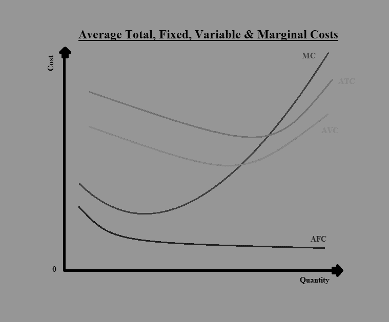
c. In the above graph, the average fixed cost is downward sloping, representing a fall in the average fixed cost in the long run.
All the other costs, i.e. average variable cost, average total cost, and the marginal cost is downward sloping in the beginning till the time it reaches its minimum and then starts sloping upwards, representing that beyond a certain limit, the average of these costs start increasing.
d. It should be noted that the marginal cost curve intersects the average variable cost when the average variable cost is at its minimum. A company should always produce this amount of goods.
Any point left to this point would mean that the cost of producing an additional quantity of a good (represented by the marginal cost curve) is less than the average variable cost of the goods. Thus, it is desirable to increase the quantity, at least up to a limit where the average cost equals the marginal cost.
1.4. Demand & Total Revenue Functions
There are basically two types of markets, i.e. perfect competition, and imperfect competition. The two markets exhibit different demand and total revenue functions.
1.4.1. Demand & Total Revenue Functions in the Perfect Competition Markets
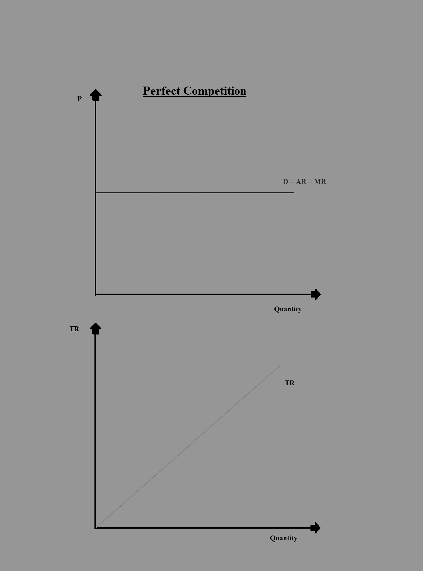
a. In perfect competition markets, the prices are fixed, and the firm can sell as much quantity as it can at this price.
b. Thus, the demand curve in such markets is a horizontal straight line, and it also equals the marginal revenue and the average revenue curve.
c. The total revenue curve is a linear, upward sloping curve with a slope of 1.
d. We can present the function in the form of a graph as follows:
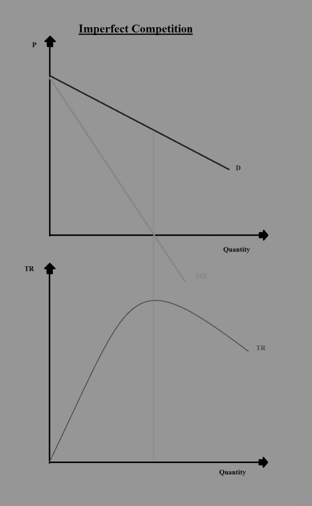
1.4.2. Demand & Total Revenue Functions in the Imperfect Competition Markets
a. In the imperfect competition market, the marginal revenue curve is downward sloping, slightly inwards of the demand curve.
b. The marginal revenue curve becomes negative after a point, indicating that after a point the additional revenues from selling the output are negative.
c. The total revenues are maximum at this point (i.e. the point at which the marginal revenues become zero).
d. This can be explained with the help of the following graph:
1.5. Profit Maximization
For identifying the points at which the profits are maximum, there could be two situations as well, i.e. one, in a perfect competition market and two, in an imperfect competition market.
1.5.1. Profit Maximization in Perfect Competition Markets
a. The firms can have the maximum profits at the point where the short-run marginal cost curve is equal to the marginal revenue curve and the short-run marginal cost is rising.
b. Consider the following figure:
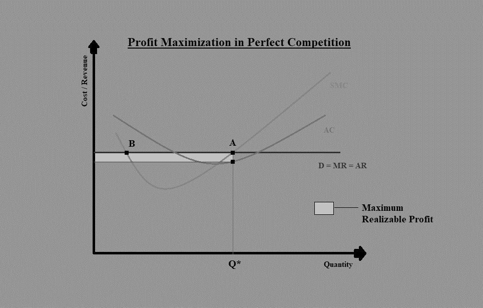
c. In the above figure, the SMC equals MR at two points A and B. However the profits would be maximum at point A, where quantity is Q*. This is mainly because, at point B, the SMC is falling, and at point A, the SMC is rising. According to the requirement, the profits are maximum at the point where SMC=MR and SMC are rising.
d. This is the point of equilibrium because, at the points to the left of point A, the additional revenues from producing and selling one more unit of the good are more than the additional cost of producing the same. And, at the points to the right of point A, the additional revenues from selling the good is less than the additional cost of producing the same.
e. At point A, the maximum profit that can be realized is represented by the shaded rectangle. The total revenues here are the average revenue at point A multiplied by the quantity, i.e. Q*. And the total cost is the average cost at the quantity level of Q* times the quantity. The difference between the same (represented by the shaded rectangle) is the maximum profit obtainable by the firm.
1.5.2. Profit Maximization in Imperfect Competition Markets
a. The condition for identifying the point of maximum profit in an imperfect competition market is the same as that in the perfect competition market, i.e. the point where SMC=MR and SMC are rising.
b. However, the shape of the demand curve, average revenue curve, and marginal revenue curve are different in this market.
c. Consider the following diagram:
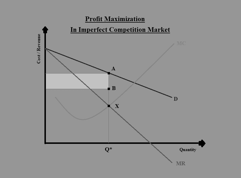
d. In the above figure, the point at which the firm can obtain the maximum profit is X. At this point, SMC=MR and SMC are rising.
The total revenue at this point is quantity times the average revenue. The average revenue for the quantity level Q* is the corresponding point lying on the demand curve, i.e. A. It indicates the price at which the firm can sell all of its quantity Q*.
Suppose the corresponding point for the quantity Q* on the average cost curve is B; the total cost of the firm would be the quantity times the average cost.
The total profit can be obtained by finding the difference between the total revenues and total cost. It is represented by the shaded rectangle in the above figure.
NOTE:
a) An important thing that needs to be answered here is that, whether at the point of equilibrium the average total cost is minimum or not? Or, to put it, in other words, is the profit maximum when the average total cost is minimum or not?
b) The answer is: not necessarily. The profit is maximum, when:
i. MR = SMC, and
ii. SMC is rising
This may not necessarily be the point where the average total cost is minimum.
1.6. Breakeven Analysis
A firm breaks even at the point where there is neither a profit nor a loss. It is the point where the total revenue equals the total costs, or the average revenue equals the average total cost.
1.6.1. Breakeven Point in Perfect Competition Market
a. Consider the following diagram:
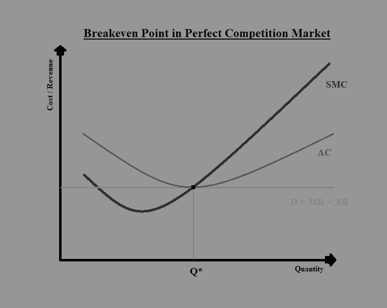
b. In the above diagram, the average cost equals the average revenue at the quantity level of Q*.
c. At this point, the average cost also intersects the average cost, and the average cost is minimum.
d. Since the average cost equals the average revenue, the total cost also equals total revenues. The profits are thus zero at this level of output.
1.6.2. Breakeven Point in Imperfect Competition Market
a. Consider the following diagram:
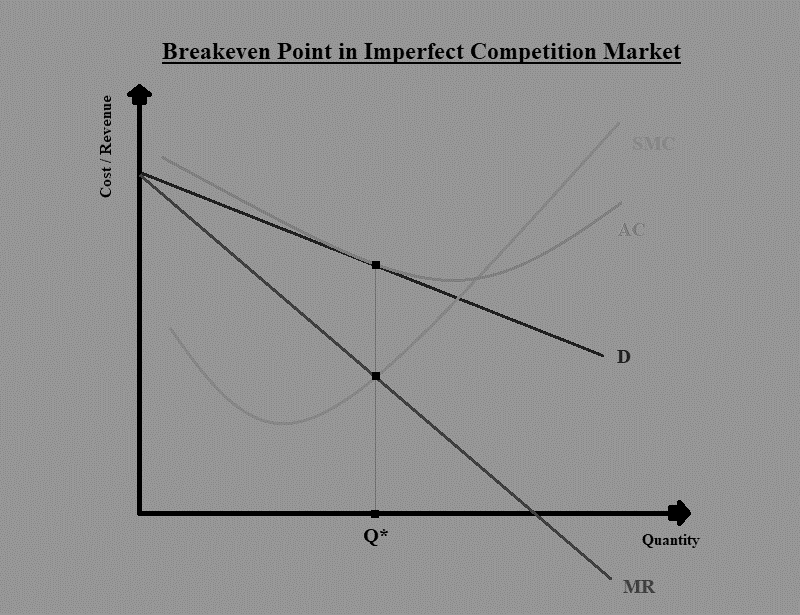
b. In the above diagram, the profit maximization is where the SMC equals the MR. This happens at the output level of Q*.
c. At the same level of output, the average revenue is the corresponding point on the demand curve. This is also the point where the average cost is equal to the average revenue. Thus, it is also the breakeven point in this case.
NOTE:
Here, the cost covered also includes the opportunity cost. Thus, the economic profit here is equal to zero.
And since it is the economic profit and not the accounting profit, the firm might still be making the normal profit.
1.7. Shutdown Decision
a. Assuming that all the fixed costs are sunk costs, a firm makes the shutdown decision in long-run and short-run as follows:
|
|
Short Run |
Long Run |
|
TR ≥ TC |
Continue |
Continue |
|
TR ≥ TVC but TR < TC |
Continue |
Exit |
|
TR < TVC |
Shut down |
Exit |
b. Thus, a firm must make the shutdown decisions as follows:
i. If the total revenue is greater than or equal to the total cost, then in both the short-run and long-run it should continue with its operations.
ii. If the total revenues are greater than or equal to the total variable costs, but the total revenues are less than the total cost, then in the short-run, it can continue, but if it continues in long run, it should make an exit.
iii. If the total revenues are less than even the total variable cost, then in the short-run the firm should shut down its operations but in long run, it should exit the business.
c. We can explain this graphically as follows:
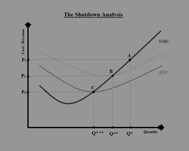
In the above figure,
i. If the prices are high, say at the level of P1, the marginal cost is rising. And, at the points to the left of A indicates that marginal revenue is higher than marginal cost, thus it would be desirable to keep producing till the firm reaches point A, at the output level of Q*. And this is the profit-maximizing point, which means that the firm is earning a profit at this price level.
ii. If the prices are slightly lower say at the level of P2. The firm would like to keep producing up to point B, i.e. the output level of Q**. At this level, the average total cost equals the average revenue. Thus, there is no profit and no loss. It is the breakeven point for the firm.
If the prices are even lower, say at the level of P3, or below. At these price levels, even if the firm produces up to the point where the marginal cost equals the marginal revenue, the average revenue would still be less than or equal to the average variable cost. Thus, it would be more advisable to shut down if the prices fall below this level. The price level of P3 or point C is, thus, the shutdown point for the firm.
1.8. Understanding Economies and Diseconomies of Scale
For understanding the economies and diseconomies of scale, it is important to understand the difference between the short-run and long-run.
In the analysis of supply, we consider two main factors of production, i.e. labor (L) and capital (K). In short-run, one of the factors of production (generally, capital) is considered as fixed, and the other (usually labor) is considered as a variable. In the long-run, we consider all the factors of production as a variable.
1.8.1. Economies of Scale
a. The total cost curves for both short-run and long-run can be presented graphically as follows:
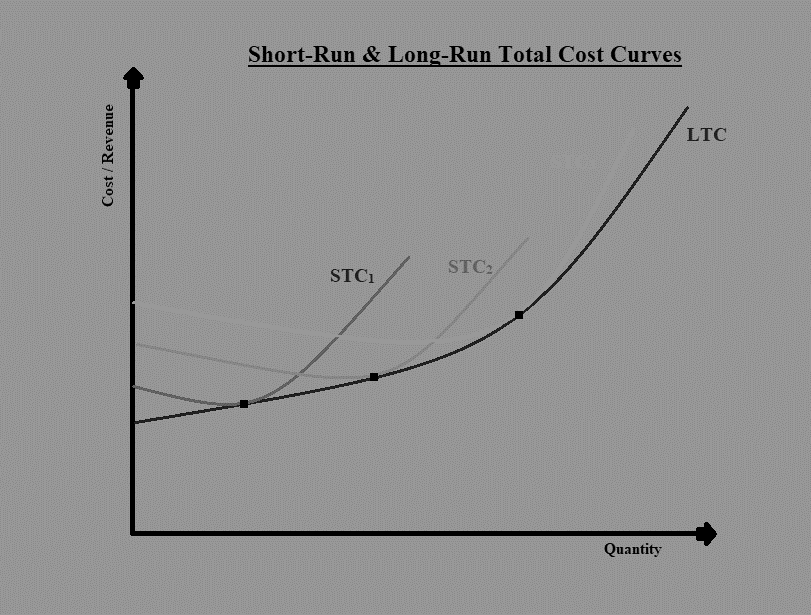
i. In the above curves, we can see that in the very short-run, the curve is STC1. In a slightly longer run, the curve extends slightly further to STC2 level, and then to STC3.
ii. The shape of the short-run total cost curve reflects the diminishing marginal return to labor.
iii. The long-run total cost curve is derived from the lowest level of STC for each level of output.
iv. The long-run total cost curve is called the envelope curve. It encompasses all the combinations of the size of the plant, technology, and capital levels.
b. That was the total cost curves in the long-run and the short-run. Now, let us consider the short-run and long-run average cost curves.
Consider the following diagram:
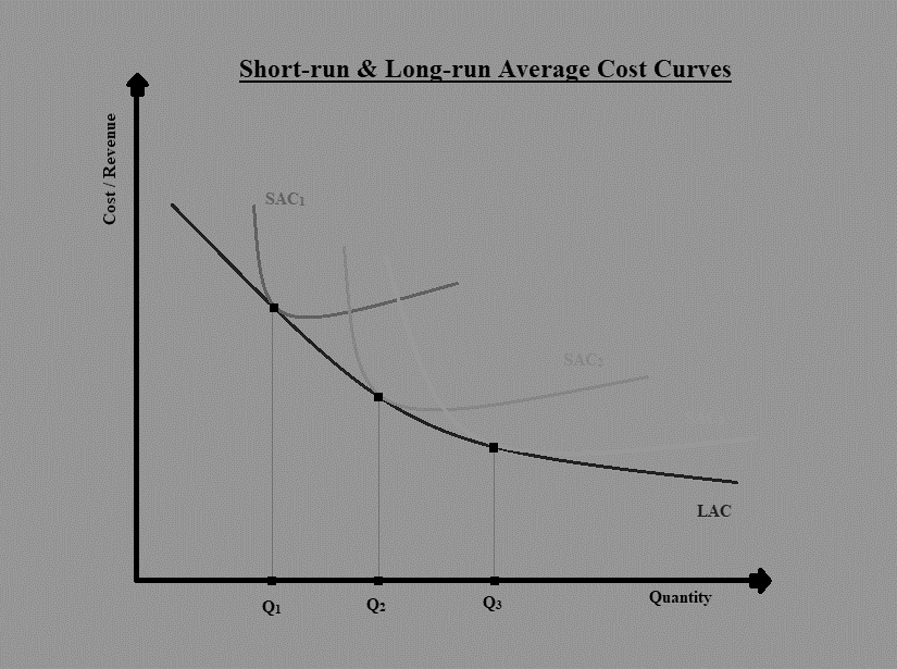
In the above diagram, we can see that:
i. In the short-run, with an increase in the level of output, there is an increase in the size of the average cost curve and a shift in the rightward direction from SAC1, to SAC2, and SAC3. With a shift, there is also a decrease in average cost at the optimal quantity level (i.e. Q1, Q2, and Q3).
ii. The long-run average cost curve is obtained by joining the optimal quantities for each of the short-run average cost curves, i.e. the minimum points in each of the short-run average cost curves.
iii. We can see from the above figure that in the long-run, the demand curve is downward sloping, indicating decreasing long-run costs per unit as output increases.
c. The decrease in long-run cost per unit with an increase in the level of outputs can be attributed to the economies of large-scale production.
The factors contributing to the economies of scale are:
i. Increase in output larger than the increase in output,
ii. Specialization in production processes,
iii. Use of more expensive, but more efficient equipment,
iv. Lower wastage costs,
v. Better use of market information,
vi. Volume discounts from the suppliers, etc.
1.8.2. Diseconomies of Scale
Beyond a certain limit, despite the increase in the scale of production, the average cost of producing the goods start increasing.
This can be seen with the help of the following diagram:
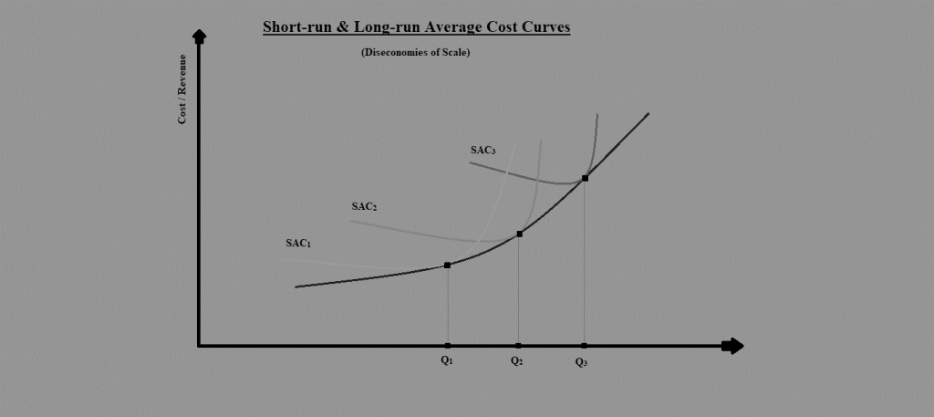
Thus, beyond a certain level of production, the long-run average cost curve becomes upward-sloping.
This can mainly be attributed to the diseconomies of scale. Some of the factors that contribute to diseconomies of scale are:
i. An increase in output is less than the increase in input,
ii. The scale of operations become too large to be able to manage efficiently,
iii. There may be duplication of processes,
iv. There may be higher labor cost,
There may be higher resource costs, etc.