a. Before discussing economic growth and its sustainability we need to understand the factors that affect the long-term economic growth and its sustainability.
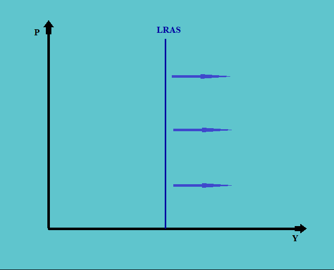
b. The long-term aggregate supply curve represents the situation of full-employment and potential GDP in the long run. Thus all the factors that work towards shifting the long-run supply curve towards the right, also are the factors causing the long-run economic growth.
c. One cannot easily estimate the long-run aggregate supply that is sustainable. However, one can use some of the proxies to estimate the same. One can calculate the long-run growth in real GDP and real GDP per capita.
d. The main factor that shifts the LRAS to the right is the additions to productive capacity.
e. Thus, for the calculation of the sustainable rate of economic growth, one needs to calculate the rate of increase in productive capacity.
f. For the sustainability of economic growth, one should look at the following important things:
i. the sources of economic growth,
ii. the stability of the inputs or the ratio of the inputs, and
iii. the sustainability of long-term growth.
1.1. The Production Function
a. In order to determine the source of economic growth, we need a production function.
b. There are basically three types of production functions: the traditional production function, the classical production function, and the neoclassical production function.
c. The traditional production function was given by Thomas Robert Malthus. According to it, the output is considered as a function of Labor. That is,
| Y = F (L) |
This model was formulated before the industrial revolution when the output was produced mainly as a result of the work done by the labor force.
d. After the industrial revolution, there was a shift in production from merely on farms and households to industries. This required a lot of capital as well. Thus, production was not just a function of labor but also capital.
Thus, the classical model recognizes the production or output as both capital and labor.
| Y = F (L,K) |
e. Then there was a shift towards the neo-classical model. In this model, the production function is further defined by another factor, i.e. A.
The production function, here, indicates a relationship between output and the inputs of technology, labor, and capital:
|
Y = A × F (L,K) Where, Y is the level of aggregate output A is the technological knowledge F indicates the functional relationship L is the quantity of labor K is the capital stock |
This is also called Solow Growth Model, named after the economist Robert Solow.
f. A, here, is the total factor productivity (TFP), which is growth in output not attributed to K or L.
g. We use the production function to link the output in an economy to the inputs.
h. Thus, we can say that GDP or long-run aggregate supply increases due to either:
i. increase in the stock of labor and stock of capital (i.e. L, K), and
ii. speed of technological changes
i. In the above model, if we consider both the variables, i.e. L and K, there will constant returns to scale (as a result of an increase in the levels of production. However, if we keep one of the inputs, i.e. either L or K, there will be diminishing the marginal productivity of the other input.
j. We can now sum up the discussion above to define the growth in potential GDP in form of an equation as follows:
| Growth in Potential GDP = Growth in Technology + WL × (Growth in labor) + WC × (Growth in Capital) |
In the above equation:
i. The growth in technology is given and is considered exogenous.
ii. Whereas, WC is the weight of capital and WL represents the weight of labor.
iii. The ratio of the weights of the two components, i.e. WC:WL shows the capital to labor ratio in the economy.
iv. The value of WL can be calculated by dividing the total value of wages paid in the economy during the year divided by the total GDP. That is
WL = W / GDP
v. The value of the weight of capital is the one minus the weight of labor. That is
Or, it can also be calculated by dividing the sum of total corporate profits, net interest income, net rental income, and depreciation, by the GDP. That is:
WC = 1 – WL
vi. The higher the ratio of a factor input in the GDP, the higher will be the impact of its growth on the growth of GDP.
WC = [Corporate Profits + Net Interest income + Net Rental Income + Depreciation] / GDP
k. We can also calculate the value of growth in per capita potential GDP from the above, which is:
| Growth in per capita potential GDP = Growth in technology + WC (growth in the labor-capital ratio) |
1.2. Sources of Growth
We have the following sources of growth in the GDP:
a. Labor Supply (Quantity): The labor force in an economy is the quantitative measure of the working hours provided by the human resource in the economy. The labor force is the participation rate of the population. It is the population belonging to the working-age who is either employed or is looking for employment.
Thus the potential size of the labor supply is the average hours worked times the labor force. That is:
Labor Supply = Labor Force × Average Hours Worked
The quality of labor supply is hugely affected by the population demography, immigration laws, daycare and child benefit policies in the country, etc.
b. Human Capital (Quality): The quality of human capital depends on the education, training, and experience of the labor force in the economy.
The quality of human capital depends upon the policies for:
i. public funding,
ii. students loan,
iii. unemployed retaining programs, etc.
c. Physical Capital Stock: The physical capital stock completely depends upon the net investment (i.e. gross investment minus the depreciation) in the capital assets of the economy.
The government can provide benefits in the form of investment tax credits, or tax deferment of abatement in case of capital investment, etc. to encourage the investment in the physical capital stock.
d. Technology: This is the most important factor that can influence the level of growth in an economy. It helps in overcoming the limitations imposed by the law of diminishing marginal productivity on the individual factors of production.
The government should provide more funding for the research and development programs, aiming at bringing new technology to the market or innovating the existing one. The government can also promote growth in technology by providing innovation tax credits.
If we recall, the formula for the growth in potential GDP was:
Growth in Potential GDP = Growth in Technology + WL × (Growth in labor) + WC × (Growth in Capital)
The term growth in technology is also called the total factor productivity. Thus we can write the equation for total factor productivity as:
TFP = Growth in Technology + WL × (Growth in labor) + WC × (Growth in Capital)
e. Natural Resources: The natural resources could be both renewable as well as non-renewable. There may be some sort of short come in the availability of these resources due to geographical or other reasons. The import can help to a large extent in overcoming such deficits.
Thus government can have policies such as free trade policies, farm subsidies, reforestation policies, etc. to promote the growth in natural resources.
f. Consider the above equation again:
Growth in Potential GDP = Growth in Technology + WL × (Growth in labor) + WC × (Growth in Capital)
In this equation, the term growth in potential GDP is unobservable. Growth in technology is exogenous and thus unobservable. And finally, for the other two components, i.e. growth in the factors, the data is not available in most of the countries.
We, thus, need some of the proxies to measure the growth. One such proxy is the calculation of labor productivity; which can be calculated as follows:
Labor Productivity = (Real GDP) / (Aggregate Hours)
Also, if we recall:
Y = A × F (L,K)
If we divide the whole equation by L, we get:
Y / L = A × F [1, K/L]
We can interpret this as “the output per worker is a function of technological change and the physical capital per worker”.
g. Now in the above equation, the term Y/L represents the level of labor productivity, which depends upon the stock of human and physical capital.
Given this, the growth of labor productivity can be calculated as:
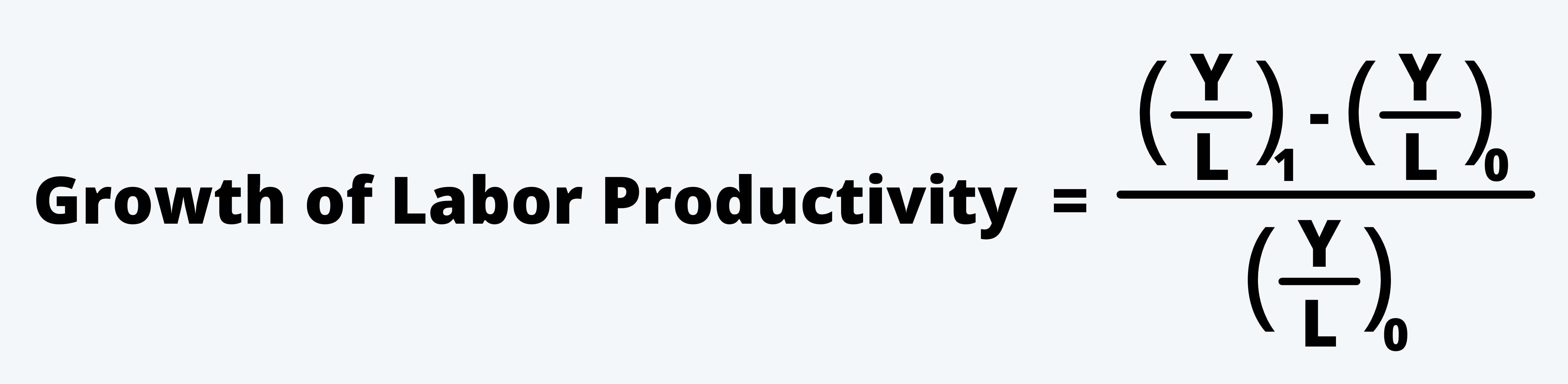
Which is the difference between labor productivity in year 1 and 0 divided by the labor productivity in year 0.
h. From the above, we can calculate the potential GDP as:
|
Potential GDP = Aggregate Hours Worked × Labor Productivity |
Also, we can calculate the potential growth rate as:
Potential Growth Rate = LT growth rate of labor force + LT labor productivity growth rate