a. The market is defined as “a group of buyers and sellers that are aware of each other and are able to agree on a price for the exchange of goods and services”.
b. As per the economists, there are four types of market structures. i.e. perfect competition, monopolistic competition, oligopoly, and monopoly.
c. There are five factors that determine the market structure; they are:
i. The number and relative size of firms supplying the product
ii. The degree of product differentiation
iii. The power of the seller with respect to the pricing decision
iv. The relative strength of barriers to the market entry and exit
v. The degree of nonprice competition
d. A summary of the four market types, based on the factors that determine these market structures are:
|
Factors |
Perfect Competition |
Monopolistic Competition |
Oligopoly |
Monopoly |
|
Number of Sellers |
Many Firms |
Many Firms |
Few Firms |
Single Firm |
|
Barriers to Entry |
Very Low |
Low |
High |
Very High |
|
Product Differentiation |
Homogeneous |
Substitutes available but differentiated |
Close substitutes or differentiated |
Unique products |
|
Non-Price Competition |
None |
Advertising and product differentiation |
Advertising and product differentiation |
Advertising |
|
Price Power |
None |
Some |
Some to significant |
Considerable |
|
Example |
Grains Market |
Soaps |
Luxury Cars |
Patented Pharmaceutical products |
e. We will discuss each market in detail in the following section.
1.1. Perfect Competition
1.1.1. Characteristics of Perfectly Competitive Markets
A perfect competition market is characterized by the following:
i. A large number of potential buyers and sellers
ii. The product offered by the sellers are virtually identical
iii. There are a few or easily surmountable barriers to entry and exit
iv. The sellers have no market pricing power
v. Non-price competition is absent
1.1.2. Demand Analysis in Perfect Competition Market
a. The market demand curve is a downward sloping curve, indicating an inverse relationship between the price of the goods and the quantity demanded, i.e. when the prices go up the demand falls and vice-a-versa.
b. A demand function is expressed as quantity as a function of price.
| Q = f (P) |
c. An inverse demand function is expressed as the price as a function of quantity.
| P = f (Q) |
d. The total revenue is price times the quantity.
| TR = P × Q = f (Q) × Q |
e. The marginal revenue is the change in total revenue due to a change in quantity produced and sold. It can be calculated by differentiating the total revenue function with respect to the quantity.
| MR = ∆TR / ∆Q |
f. The demand curve and the marginal revenue curve can be presented as follows on a graph:
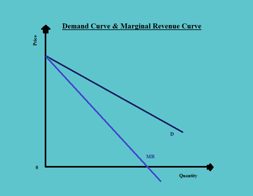
g. The marginal revenue is a function of price and the own-price elasticity of the product. The function can be written as:
| MR = P [ 1 – (1/E)] |
1.1.3. Supply Analysis in Perfectly Competitive Markets
a. According to the basic supply function, when market prices increase, the firms supply greater quantities.
b. The market supply curve is the sum of the supply curves of the individual firms.
1.1.4. Optimal Price and Output in Perfectly Competitive Markets
a. In order to attain the equilibrium and optimal price and output in perfectly competitive markets, one should equate the market demand and supply.
b. Therefore, if the supply function is:
P = f (QS)
And, if the demands’ function is:
P = f (QD)
Then, the equilibrium can be attained by solving the equation:
| f (QS) = f (QD) |
c. Diagrammatically, the equilibrium is attained at the point where the demand curve intersects the supply curve.

d. The one depicted in the above diagram is the market equilibrium. This equilibrium level helps in identifying the price level at which the market demand equals the quantity that would be supplied.
But, at this given price the optimal amount of goods supplied by the individual firms, that would maximize the profits can be identified by finding the level of production and sale where the marginal cost is equal to the marginal revenue and the marginal cost curve is rising.
Consider the following diagram:
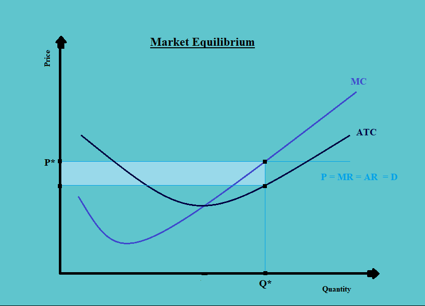
We find the following:
i. Generally, the cost curves (including the marginal cost and average total cost curves) are U-shaped because of the law of diminishing marginal returns.
ii. The average total cost intersects the marginal cost curve when the average total cost is minimum.
iii. The profits are maximized when the marginal revenue is equal to the marginal cost curve. Thus, each firm will produce up to the level where their marginal revenue equals the marginal cost.
iv. The marginal cost curve starting from the point where the average total cost intersects the marginal cost curve is also the supply curve of the firm. This is mainly because; a firm will only supply the quantity where the marginal cost equals the marginal revenue (or the price in the perfect competition market). But, if the price falls below the average total cost, the firm would rather shut down.
v. The economic profit earned by the firm during the process is the difference between the marginal cost and the average cost times the quantity supplied. This is shown by the shaded region above.
1.1.5. Factors Affecting the Long-Run Equilibrium in Perfectly Competitive Markets
a. In the above figure, we have seen that the firm is earning an economic profit at the existing market price level. But, if the firms in any market are earning economic profits greater than zero, then other firms will enter the market, eying the same.
And when more firms enter the market, the supply increases, and the market supply curve shift rightwards, as in the figure below: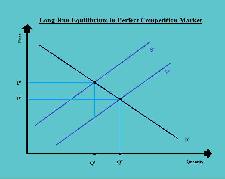
We can see in the above figure, that as a result of an increase in supply, the supply curve shifts to the right. This shift in the supply curve brings the prices down until the economic profits of the firms become zero.
b. The fall in the price will continue until it reaches the point where for the firms the average total cost is zero. And there is no economic profit for the firms, as shown in the figure below:
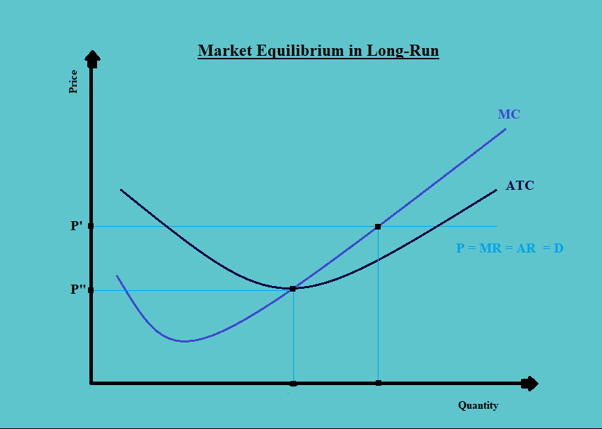
c. However, if the prices in the market are so low that the firms are making losses, then the firms will exit the market, reducing the supply, and thus the price will rise up to the level where there is neither an economic profit nor a loss.
d. Thus in the long-run, the marginal cost is equal to the marginal revenue and both equals the average total cost and price.
1.2. Monopolistic Competition
1.2.1. Characteristics of Monopolistic Competition Market
A monopolistic competition market is characterized by:
a. A large number of potential buyers and sellers
b. The products offered by each seller in the market are close substitutes of the products offered by the other firms, and sellers try to differentiate their product
c. Entry to and exit from the market is possible at a very low cost
d. Firms do have some purchasing power
e. Suppliers differentiate their products through advertising and other nonprice strategies
1.2.2. Demand Analysis in Monopolistically Competitive Markets
a. In a monopolistically competitive market, the demand curves are downward sloping for each of the firms. The main reason behind this is that each firm in such a market has a say in pricing decisions, through market differentiation. Thus, the price of the product does affect its demand.
b. The marginal revenue curve is also downward sloping and slightly steeper and inward of the demand curve.
c. Consider the following figure:
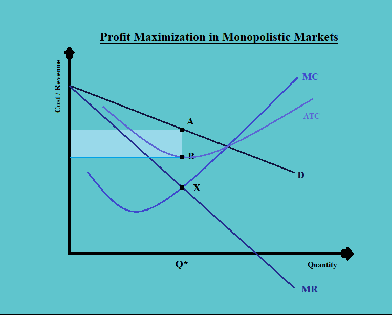
d. The profit-maximizing quantity is the one where the marginal revenue equals the marginal cost, i.e. at the quantity level of Q* in the above figure.
e. The economic profit of the firm is represented by the shaded region. It is the difference between the price and the average total cost times the quantity.
1.2.3. Supply Analysis and Optimal Output in a Monopolistic Market
a. As seen above, the level of output is based on the fact where marginal revenue equals marginal cost, and the price is based on the demand by the customers.
b. Unlike the perfect competition markets, the supply function is not very well defined in monopolistic markets. This is mainly because the demand function in the perfect is a straight line, as the prices are fixed by the market demand and supply. Whereas, the demand curve and marginal revenue curve in the perfect competition market are downward sloping and the quantity supplied is dependent on the same.
c. The prices in the monopolistic competition are higher and the quantity demanded is lower.
1.2.4. Factors Affecting Long-Run Equilibrium in Monopolistic Competitive Markets
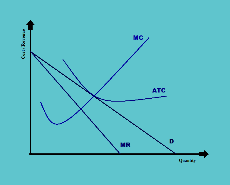
a. In the long run, the economic profit of the firms in monopolistic competitive markets is zero.
b. This is mainly because; if a firm is earning economic profits, more firms will enter the industry and this will result in the firm’s demand curve moving inwards; and vice-versa in the case of losses. This transition will continue till the time there is zero economic profit.
c. At zero economic profit, the firm’s cost, revenue, and profit structure would be as follows:
1.3. Oligopoly
1.3.1. Characteristics of Oligopoly Markets
a. There are a small number of potential sellers.
b. The products offered by each seller are close substitutes for the products offered by the other firms. And, these products may be differentiated by brand or homogeneous and unbranded products.
c. Entry into the market is difficult, with fairly high costs and significant barriers to competition.
d. Firms typically have substantial pricing power.
e. Products are often highly differentiated through marketing, features, and other non-price strategies.
f. The price depends on the pricing of competitors and the assumptions made regarding competitors’ reactions to price changes. There is also a temptation amongst the firms having the pricing power to collude, form a cartel, and set a higher price.
1.3.2. Demand Analysis and Pricing Strategies in Oligopoly Markets
a. There could be two situations in an oligopoly market, i.e. if the firms collude or if they don’t.
b. If the firms collude, the aggregate demand curve of the market is divided by the individual production participants or the firms within the market. By entering into the agreement to share the demand and setting the prices accordingly, the industry can attain the prices otherwise attainable by the monopoly.
c. If the firms do not collude, each of the firms in the industry faces an individual demand curve and the market demand curve will depend on the pricing strategies.
There are three different types of pricing strategies that may be employed by the firms in the industry. These are:
i. Pricing interdependence,
ii. Cournot assumption, and
iii. Nash Equilibrium.
d. These are discussed in detail in the following section.
1.3.2.1. Pricing Interdependence
a. This strategy implies that the prices of the firms are interdependent and thus there is a kinked demand curve.
b. According to this strategy:
i. If there is a price increase in the market, the firm may not follow the suit, and thus will enjoy the benefits of increased demand due to the substitution
ii. However, if there is a decrease in industry prices, the firm will have to cut the prices in response, in order to remain in the league.
c. This would result in a kinked demand curve and a broken marginal revenue curve. This can be explained with the help of the following figure:
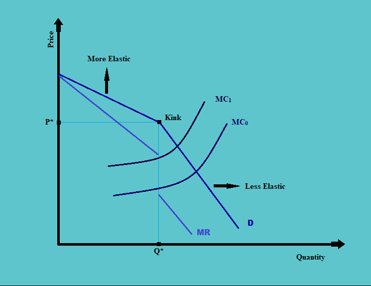
Assume that the industry has two firms (i.e. duopoly) and each firm is following a pricing interdependence strategy. The product is currently trading at the price P*.
Now, suppose that the second firm increases the price. In this situation, the first firm will not increase its price; its price remains the same. Now, the consumers would make a shift to the first firm, increasing its demand manifold due to the substitution effect.
However, if the second firm decreases the price; as a corrective measure, the first firm will also decrease its price. There will be an increase in the demand for the product due to a fall in the price. But the change in demand will not be as much as in the case of an increase in price because there is no substitution effect; the increase is only a result of the income effect.
Thus there is a kink in the demand curve, and the marginal revenue curve is broken.
d. There are two things that need to be noticed about this model, i.e.:
i. This model explains the stable price (i.e. P* in the above diagram) and the effect of deviation from it.
ii. But, this model does not explain what this stable price should be, or how we arrive at this price.
1.3.2.2. Cournot Assumption
a. The main premise of Cournot’s assumption is that ‘each firm determines the profit-maximizing quantity assuming the other firm’s output will not change’.
b. According to this strategy, each firm attempts to maximize its own profit, assuming that the other firms in the industry will continue their production at the current level. According to this model, this pattern continues till each firm in the industry reaches its long-run equilibrium.
c. Thus, in the long-run, the change in price or quantity will not increase the profits.
d. The prices under different conditions would be as follows:
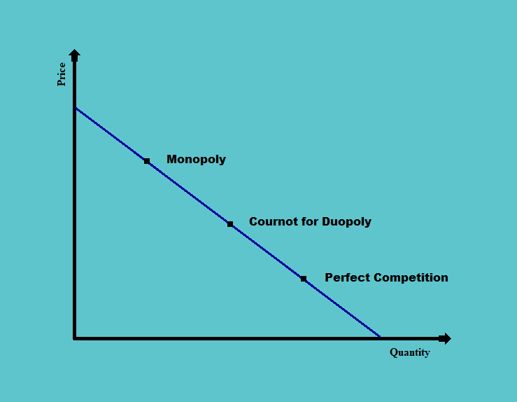
Under monopoly, the industry would be able to set the highest price of the product. The prices are least under perfect competition; under oligopoly, it lies in between. And as the number of firms in an oligopoly increase, the equilibrium point moves closer to the perfect competition.
1.3.2.3. Nash Equilibrium
a. According to the Nash Equilibrium, the firms arrive at an equilibrium strategy after considering the actions of the other firms (interdependence); there is no incentive for any firm to deviate from the Nash equilibrium.
b. The basic assumption of this equilibrium is that the firms do not cooperate/collude.
c. Suppose there are two firms A and B, selling similar products. Each of the companies can employ a high-price strategy or a low-price strategy.
The strategies and the respective profit for each firm are shown in the following matrix:
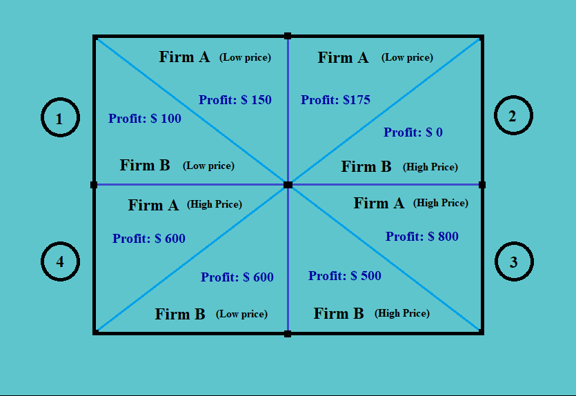
i. In the above figure, there are four matrices. The firms could be in either of the matrices, to begin with.
ii. In the long-run, the firms will always reach matrix 4.
iii. Suppose both the firms start off with a position in matrix 1, i.e. with both the firms having a low The firm A assumes that the firm B will increase its price (which is quite unlikely, as it results in zero profit for firm B, in case firm A doesn’t increase the price), and it decides not to change the price; it would still be in a better position than before, earning a higher profit of $175, in comparison to $ 150 earlier.
iv. However, if firm A also increases the price, in response (which is more likely, as it can increase the profits manifold by doing so), both the firms can have a higher profit of $ 800 and $ 500 respectively. Both the firms reach matrix 3 by doing so.
v. If both the firms start off with a higher price, i.e. in matrix 3, and firm B assumes that firm A will maintain the same level of prices, the best alternative for firm B would be to reduce the price and reach matrix 4. This way it will increase its profit from $ 500 to $ 600, despite the total industry profit being lesser than before.
vi. From firm B’s perspective, it is always better to maintain a low price, whether firm A increases the price or not.
d. Can both the firms be better off if they collide? Yes, definitely, if both the firms collude and maintain a high price, they would be better off in terms of overall higher profit for the firm.
e. The factors that affect the chances of successful collusion are:
i. Number and size of sellers,
ii. The similarity of products,
iii. Cost structure,
iv. Order size and frequency,
v. Retaliation, and
vi. The degree of external competition.
1.3.3. Supply Analysis in Oligopoly Markets
a. Like the monopolistic competition, in the oligopoly as well, the supply function is not well defined.
b. We cannot determine the output and price without considering a demand function.
c. But, like other market functions, the profit is maximized where marginal revenue equals the marginal cost. Thus, the quantity produced must be such that the marginal revenue equals the marginal cost.
d. The equilibrium price is based on the demand curve.
Suppose, in an oligopoly market we have one firm which has a significantly lower cost of production than its competitors and a 45% share of the market. This firm is the market leader or the dominant firm, along with the five other players in the market.
Now, consider the following figure:
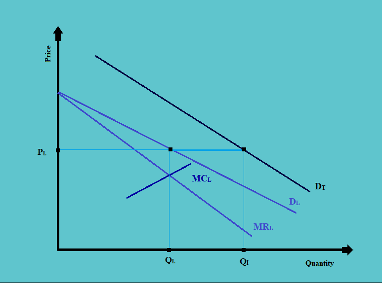
i. In the above figure, the line DT represents the total demand curve of the industry, DL is the demand curve of the market leader or the dominant firm, MRL is the marginal revenue curve of the leader, and the MCL is the marginal cost curve of the leader.
ii. The firm will supply and produce the quantity up to the point QL, where the marginal cost of the firm equals its marginal revenue. The price for this quantity can be decided based on the demands curve, which lies on the point PL.
iii. The other firms in the industry will take this price. This is mainly because, if the other firms increase the price, doing so would mean transferring the demand to the market leader.
Also, the other firms cannot decrease the price because the market leader already enjoys the economies of scale and is a low-cost producer already.
iv. Since, the leader is the low-cost producer, therefore as the difference between the market demand curve and the firm’s demand curve keeps on decreasing as the prices get When the prices keep reducing the demand will keep on shifting towards the market leader.
1.3.4. Optimal Price and Output
There is no single optimum price and output model that works for all oligopoly market situations.
1.3.5. Factors Affecting Long-Run Equilibrium
Long-run economic profits are possible but empirical evidence suggests that over time the market share of dominant firms declines.
1.4. Monopoly
1.4.1. Characteristics of a Monopoly Market
A monopoly market is characterized by the following:
a. A single seller of a highly differentiated product.
b. No close substitute for the product offered by the seller.
c. Significant barriers to entry.
d. Considerable pricing power in the hands of suppliers.
e. The product is differentiated through non-price strategies such as advertising.
1.4.2. What is a natural monopoly?
A natural monopoly is one where due to the high scale of production, the cost of the product decreases for the supplier. The low cost of production of the monopolist makes it extremely competitive for the new entrants to survive in the market; thus creating a natural monopoly for the already existing player.
1.4.3. How are monopolies created?
The monopolies may not only be natural, but they could also be created through one of the following:
a. Patent or copyrights,
b. Control over critical resources,
c. Government authorization,
d. Strong brand loyalty creates high barriers to entry,
e. The network effect, etc.
1.4.4. Demand Analysis in Monopoly Markets
a. The demand curve under a monopoly market is downward sloping. This is mainly because, even in the market with one supplier, the demand for the product is dependent on its price.
b. The demand function can be written in the form of quantity as a function of price; or alternatively, as the price as the function of quantity. That is:
|
Q = f (P) or, P = f (Q) |
c. The total revenues of a firm are the quantity times the price of the product. It can be written as:
| TR = P × Q = f (Q) × Q |
d. And the marginal revenue of a firm is the derivative of the total revenue function, i.e. change in the total revenue for each change in the quantity.
| MR = ∆TR / ∆Q |
e. The average revenue is the total revenue divided by the quantity.
| AR = TR / Q |
f. Diagrammatically, the demand curve, marginal revenue curve, and average revenue curve can be shown as follows:
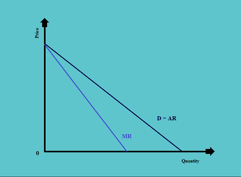
In the above diagram:
i. The demand curve is downward sloping.
ii. The average revenue curve is equal to the demand curve, as the average revenue is equal to the respective price at each level of quantity demanded.
iii. The marginal revenue is also downward sloping but a little steeper than the demand curve.
1.4.5. Supply Analysis in Monopoly Market
a. The total cost curve is a function of quantity supplied, as the total cost of production is directly related to the quantity to be produced.
b. The marginal cost is the first differential of the total cost function. That is, it represents the change in total cost for every change in the quantity.
c. The profit-maximizing level of output is the level at which the marginal cost equals marginal revenue.
d. Price is based on the demand curve. It is the price that the consumers are willing to pay at the level of quantity where the marginal cost equals the marginal revenue.
e. This can be explained with the help of the following diagram.
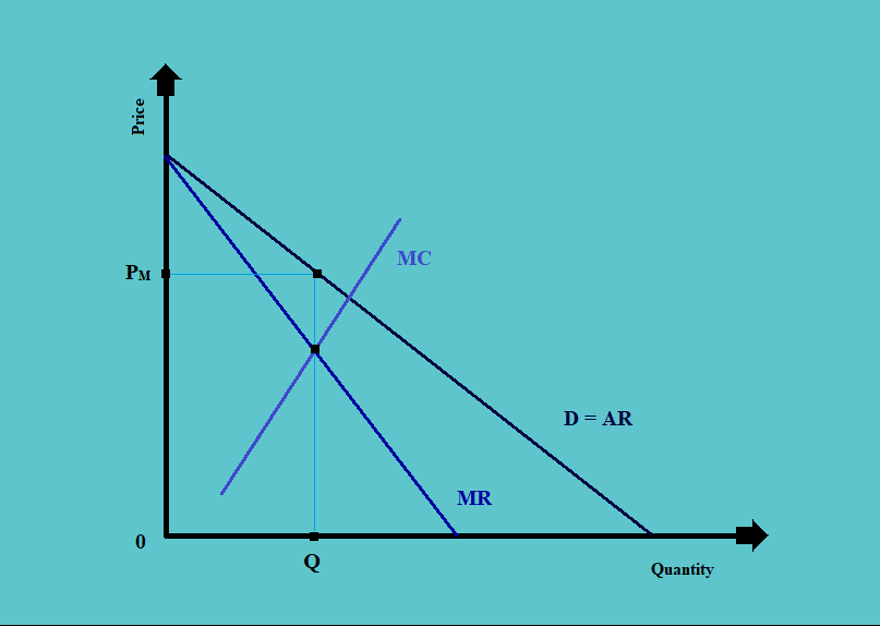
1.4.6. Optimal Price and Output in Monopoly Market
a. As stated, the optimal output exists at the point where marginal revenue equals the marginal cost.
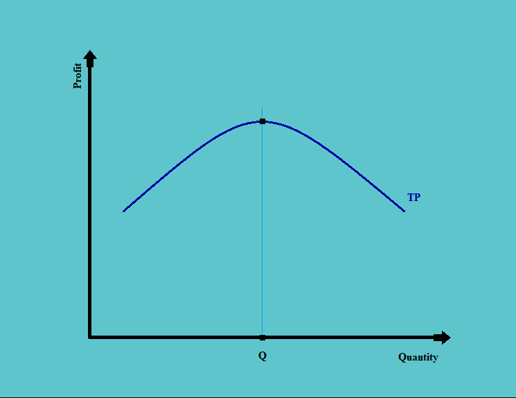
b. The profit-maximizing output level is also the point where the marginal profit (or change in profit per unit change in the output) equals zero.
c. The marginal revenue is the function of price and its own price elasticity.
| MR = P [1 – (1/E)] |
d. The condition for profit maximization is that the marginal revenue should equal the marginal cost (i.e. MR=MC). Therefore,
| MC = P [1 – (1/E)] |
e. Solving the above equation for the price, the profit-maximizing price should be:
| P = MC / [1 – (1/E)] |
1.4.7. Natural Monopoly in a Regulated Pricing Environment
a. The average cost of production in a natural monopoly falls over a relevant range of consumer demand.
b. Consider the following diagram:
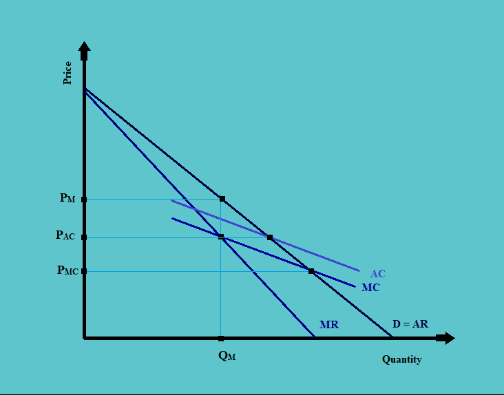
In the above diagram:
i. The profit-maximizing output happens at the point where MR = MC, i.e. QM. At this point, the price is PM.
ii. If the price is set at the average cost level, i.e. PAC, there will be no-profit-no-loss.
iii. If however, the price is set at the level where the marginal cost equals the average revenue, there will be an economic loss.
c. The government regulation may attempt to improve the resource allocation by requiring the average cost pricing or marginal cost pricing.
1.4.8. Price Discrimination and Consumer Surplus
a. Monopolists have considerable pricing power and may charge consumers in different ways. There are three different ways of price discrimination in a monopoly market.
b. First-degree price discrimination is a method of price discrimination where the consumer is charged the maximum that he is willing to pay.
That is, say if a consumer is willing to pay $ 100 for the first unit of product that he is buying he would be charged $100 for that unit. For the second unit, if the consumer will be willing to pay only $ 90, he would be charged the same; and so on.
In such cases, there is no consumer surplus.
c. In second-degree price discrimination, the consumer is charged differently based on how much he values the product.
d. In the third-degree price discrimination, the consumers are segregated based on their demographic or other traits, and a different price is charged to each of such categories based on the product’s utility to them.
1.4.9. Factors Affecting Long-Run Equilibrium in Monopoly Markets
a. Unregulated monopolies can and usually do earn economic profits in the long run.
b. For the regulated monopolies, there can be several possible solutions, such as:
i. The regulator may set the price up to the level where it is equal to the marginal cost.
ii. There may be national ownership, wherein a national entity may take over the monopoly.
iii. There may be a government entity authorized to take over the monopoly.
iv. The monopoly firm may be franchised through a bidding war.