a.  The business cycle is a fluctuation in economic activity around the long-term trend line, experienced by the economy over a period of time.

b.  Factors that may affect business cycles are some of the same factors that affect economic growth (e.g., labor productivity, money supply, inflation, and technology).

c.  The general characteristics of a business cycle are:

     i.  They are typical in economies that rely on business enterprises.

    ii.  There are alternating phases of expansion and contraction.

   iii.  Phases occur throughout the economy, most often simultaneously.

   iv.  Phases reoccur but vary in duration and intensity.

1.1.         Phases of Business Cycles

a.  Consider the following diagram:

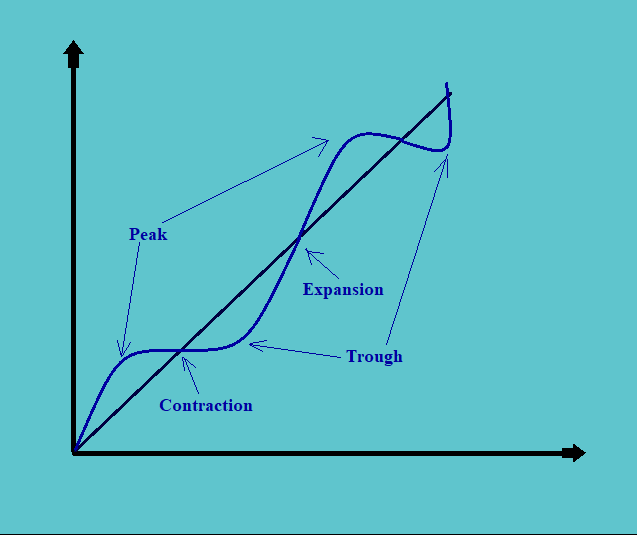
The above diagram shows the business cycles in an economy over a period of time.

b.  A business cycle consists of an expansionary period and a contractionary period. An expansion occurs after a low point (the trough) and a contraction occurs after the highest point (the peak).

c.  In reality, however, the rising part of the business cycle can be divided into two parts:

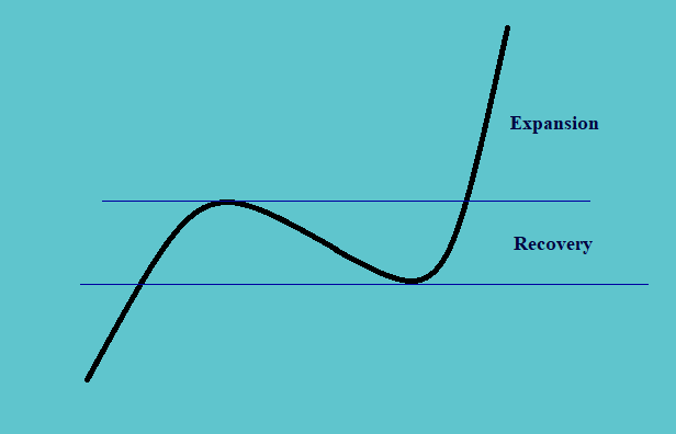
     i.  When the trendline is rising, starting from the trough up to the point where it reaches the level of the previous peak, it is called the recovery.

    ii.  Post recovery, the further rise is called the expansion.

d.  In the above figure of the business cycles, we can see some symmetry in the phases of the cycles, but in reality:

     i.  the phases are not so symmetrical, and

    ii.  they are recurrent but not periodic, in the sense that they may vary in duration and intensity.

e.  The downturn in economic activity may also either turn into either recession or depression.

    i.  The recession is a general contraction in output. It is broad-based and generally for two quarters.

    ii.  A contraction is referred to as depression if severe and if aggregate activity declines.

f.  The business cycle can be described in terms of capital spending inventory levels, consumer behavior, housing sector behavior, and external trade.

g.  We can summarize the business cycles through the following table:

1.2.         Leads Vs. Lags

a.  There are different types of economic indicators for the trends in the economy.

b.  Of these, some of them may:

     i.  lag in their indications,

    ii.  be coincident in their predictions, or

   iii.  may lead to their predictions.

c.  The financial markets generally lead the economy. In the sense that, some of the other economic indicators might show the signs of contractions heading towards trough, but the financial markets at the same time may already show the signs of recovery.
The financial markets are not just the indicators of where the economy stands today, but they indicate where it is headed in a couple of quarters from now.

d.  The monetary and fiscal policy, on the other hand, works with a lag. They look at the current economic situation; make anticipation of the future and works towards managing the same.

e.  The indications by the leading economic indicators are subject to revisions at some future point in time. These revisions may happen after a couple of months or even up to a year later.

f.  There is a further complication to these indicators’ predictions; the behavior (whether induced by an indicator or otherwise) may also lead or lag an economic trend.

1.3.         Resource Use Through Business Cycles

Consider the following diagram:

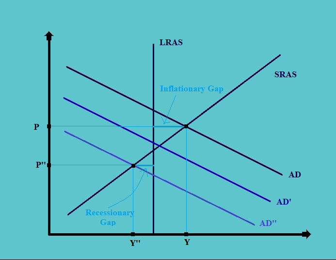
In the above figure:

a.  The original equilibrium is at the output level Y and price P, where the aggregate demand curve, AD equals the short-run aggregate supply curve, SRAS.

b.  However, this equilibrium is not at a point on the long-run aggregate supply curve, LRAS. The supply at this level is more than the one required in the long run, and this difference indicates the short-run inflationary gap. This may be considered a peak.

c.  Due to the inflationary gap, the inventories start to build up and production slows down, shifting the aggregate demand curve from AD to AD’. In the case of the long legs, the layoffs also begin to increase.

d.  This can be called the contractionary phase, and is characterized by the following:

     i.  sluggish inventory turnover,

    ii.  delayed equipment purchases,

   iii.  reduced production,

   iv.  cuts in overtime and shorter workweeks.

e.  The contraction phase induces the consumer precautionary savings, bringing the aggregate demand inwards further from AD’ to AD’’.

f.  At this point, the short-run aggregate supply is less than the long-run aggregate supply; creating a situation of the recessionary gap.

g.  The whole process is called the aggregate demand-led contraction. Here the prices in the economy also decrease from P to P”.

Now consider the following figure:

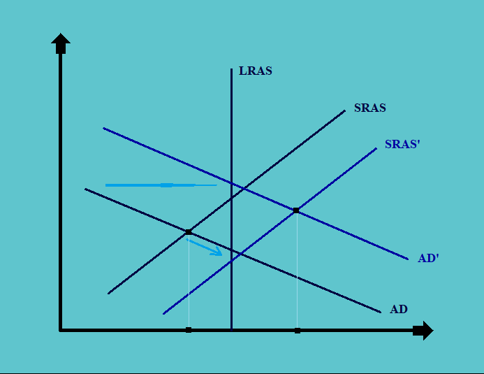
h.  As a result of aggregate demand-led contraction, the prices fall to a great extent.

i.  The low prices begin to induce the demand, and there is a movement rightwards on the demand curve AD.

j.  Further, low demand induces low-interest rates, which results in increased demand for credit. This results in a higher demand for high value and durable goods, shifting the aggregate demand itself from AD to AD’.

k.  To compensate for the increased demand, the production also increases, shifting the short-run aggregate supply curve from SRAS to SRAS’. This also increases the total output in the economy from Y to Y’, however, the impact on the price depends on the magnitude of the shift in the aggregate supply curve.

l.  The whole process is called aggregate demand-led expansion.

1.4.         Impact of Different Phases on The Aggregate Demand

a.  The beginning of the phase where the aggregate demand begins to fall or when the contraction phase begins is characterized by new orders being halted, especially for the non-durables and light equipment.

b.  The phase when the aggregate demand reaches its low or recession is mainly characterized by the major capital project being put on hold. There is a huge drop in the demand for heavy equipment.

c.  The expansion phase, in the beginning, is characterized by a pick-up in the IT investments. This phase is characterized by the investments in the project that will improve efficiency rather than capacity.

d.  The peak phase of the business cycle is mainly characterized by capacity expansion, high demand for heavy equipment and structure, etc. The capacity utilization in this phase is in the range of 80-88% range.

1.5.         Impact of Different Phases on The Inventory

a.  The beginning of the phase where the aggregate demand begins to fall or when the contraction phase begins is characterized by a sales drop. This causes the inventory to build up and there is an increase in the inventory accumulation ratio.
As a corrective step, there is a cut in production below the sales levels.

b.  The phase when the aggregate demand reaches its low or recession to when the expansion phase begins is mainly characterized by a drop in the inventory-sale ratio followed by a drop in the inventory levels.
Here the production begins to rise, maybe above the sale levels, as a process of inventory rebuilding.

c.  From the beginning of the late expansion up to the peak phase of the business, the cycle is mainly characterized by the increase in sales, however, the inventory is stable. Thus there is a fall in the inventory-sale There is a surge in production to above the sales level if the inventories are low, and there is a measured increase in the production if the inventories levels are okay.

1.6.         Impact of Phases of Business Cycles on The Consumer Behavior

Consumer behavior generally is affected by the trends in the economy. Hence, there are certain traits of consumer behavior that act as the leading indicators of the business cycles. Some of them are:

a.  Retail Sales: The demand for durable goods is one of the leading indicators of the business cycles. It goes up with the uptrend and vice-versa.
The demand for the non-durables and the services are also considered as the indicators, however not as strong as the durables, as they are considered as staples.

b.  Consumer Confidence and Sentiments: It is also one of the very good indicators of the business cycles. If the consumers are confident they spend more on heavy and durable goods. On a contrary, if they are not, they spend only on staples and prefer to save more.

c.  Income: Income, especially the disposable one, is more correlated with the consumption of non-durables and services.

d.  Savings: Increase in the levels of savings, may indicate future caution. Also, the stock of savings is a good indicator of how much the consumption will be in the future, without the need for income.

1.7.         Impact of Phases of Business Cycles on The Housing Sector Behavior

a.  The housing sector is a very interest-rate sensitive sector. And, it is a sector that in turn also affects and stimulates the behavior of the other industries which provide the raw material to the housing industry, and the demand for labor and employment conditions in the economy.

b.  To have a detailed insight into the behavior of the housing sector, one needs to look into the following:

     i.  The data for new and existing home sales. It gives a great idea about the demand for the housing sector in the economy and the inventory in this sector.

    ii.  The housing price index (HPI), which is a measure of the affordability of housing in an economy. This index is calculated by dividing the income by the average housing prices in an economy.

c.  A typical graph for the movements of interest rates and HPI in an economy is as follows:

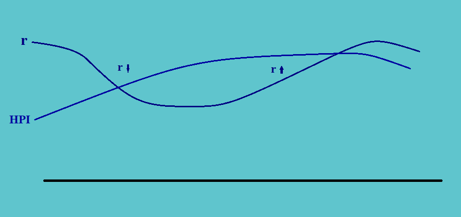
     i.  When the rate of interest is falling, housing becomes more affordable to the consumers. This induces the HPI index to rise.

    ii.  When the interest rates start rising as well, there is an increase in the prices of housing. But the interest rates start rising only in response to the increase in income in the economy.
And, since the increase in income is more than the rise in housing prices, there is still an increase in the HPI index.

   iii.  However, when the interest has risen so much that it begins to work against the income, there is a fall in the HPI index. At this point, the ratio works against the prices as the rates rise and the affordability becomes low.

   iv.  The construction of new houses generally works in correlation with the interest rates.

1.8.         Impact of Phases of Business Cycles on The External Trade Sector Behavior

a.  The imports of a country are dependent upon the income levels in that country or its Thus:

     i.  When the GDP of an economy is falling, its import levels too

    ii.  And, when the GDP of a country is rising, its imports rise as well.

b.  The exports of an economy are dependent upon the economic conditions in the countries which form the biggest consumer of its exports. Thus:

     i.  When the GDP of the country/countries that form its biggest importers decline, the export levels of the economy also decline.

    ii.  And when the GDP of such countries rises, the export levels of the economy also increase.

c.  Thus we may not be able to track the net export (i.e. exports minus the imports) through the domestic business cycles only.

d.  Another factor that has an impact on the levels of net exports is the foreign exchange rates.

     i.  When the foreign exchange rates are low there is a high demand for imports and low levels of export, thus a very low level of net exports.

    ii.  When the foreign exchange rates are high there is a low demand for imports and high levels of export, thus a very high level of net exports.