Before we start with the demand concepts, it is important to understand what demand is. Demand is the quantity of a commodity, goods, or service that the consumer is willing and able to buy at a certain price.

1.1.           Law of Demand

a.  The law of demand is a microeconomic law.

b.  It states that:

     i.  all the other things being constant,

    ii.  if the price of goods or services increases,

   iii.  the quantity demanded of those goods and services decreases,

   iv.  and vice-a-versa.

c.  This is mainly because as the price of the goods rises, the buyers will choose to buy less of those goods; and as the price decreases, they buy more.

1.2.           Demand Function

a.  The demand function is a mathematical expression of the relationship between all the factors that impact the willingness and the ability of a consumer to demand a particular good, and the quantity demanded.

b.  There are many factors that affect the demand for goods, such as, the price of that good, the income levels, the price of other goods (such as substitute goods, complementary goods, etc.).

c.  Thus, the equation of a basic demand function for a good A can be written as:

d.  For example, say the demand for tea in a particular city has the following function:

Q_D = 15 – 0.4P + 0.2I – 0.3P_s

Where, Q_D is the quantity demanded, ‘P’ is the price of tea, ‘I’ is the income level of the consumers, and ‘P_s’ is the price of a complementary good (i.e. sugar).

If we are told that the average income levels in the city are $ 1500 and the price of the complementary good is $ 40, then a simplified linear demand function would be:

Q_D = 303 – 0.4P

e.  Thus, a simplified linear demand function is the amount of quantity demanded stated as a function of only one factor affecting it, mainly, the price of that good.

1.2.1.       Inverse Demand Function

a.  As seen above, a linear demand function states the quantity demanded of a good as a function of price.

b.  The inverse demand function reverses the equation and states the price of a good as a function of goods demanded.

c.  Thus, for the above demand function, the inverse demand function is:

P = 757.5 – 2.5Q

1.3.           Demand Curve

a.  A demand curve is a graph representing the linear relationship as depicted in the demand function.

b.  We can draw a demand curve using the above inverse demand function as follows:

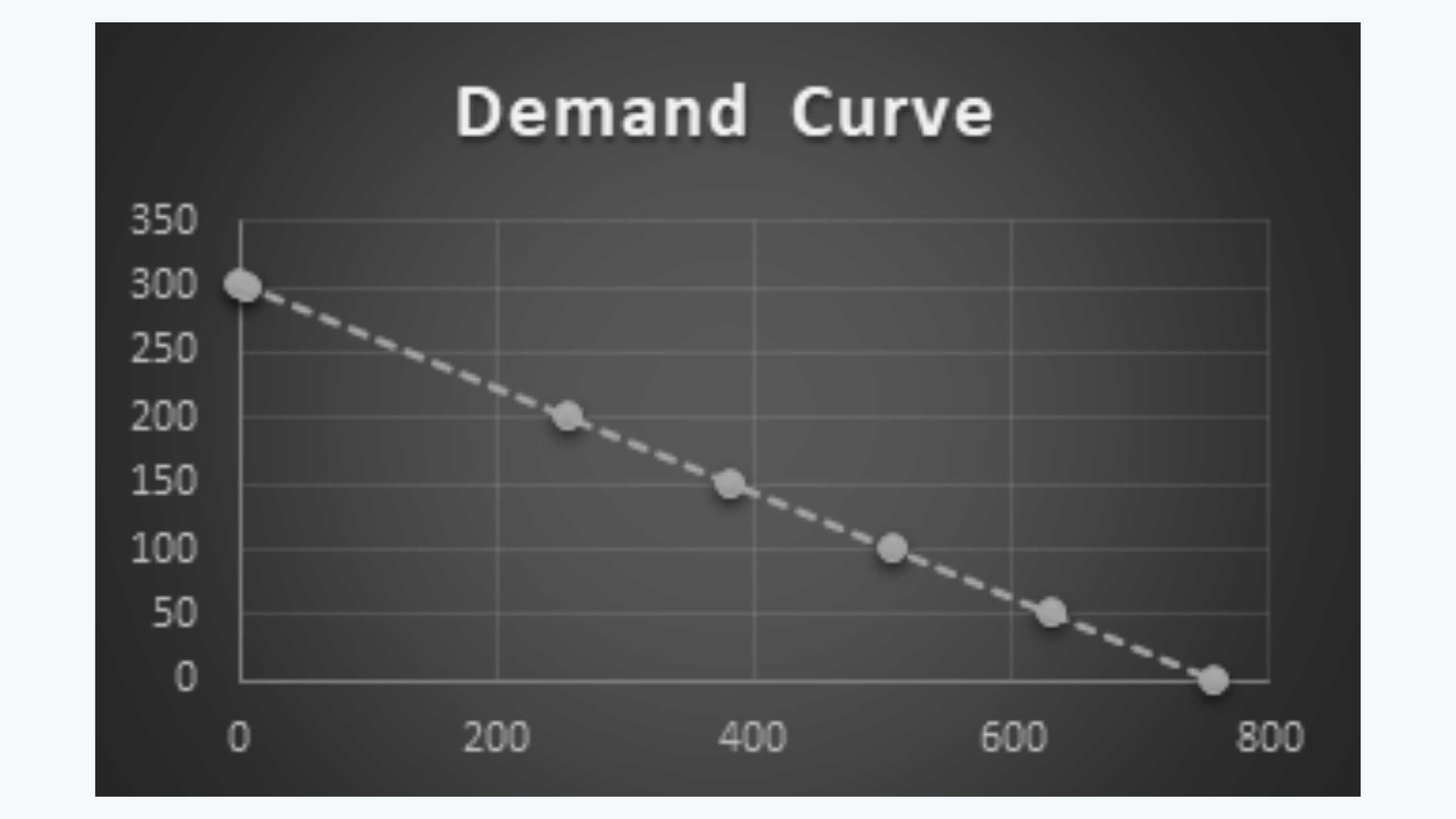
c.  The above demand curve shows the linear relationship between the quantities of tea demanded at different prices. According to this demand curve, when the price of tea is $ 0, 757.5 units of quantity will be demanded; and when the price is $ 303, the demand for tea will become 0.

d.  The coefficient of Q, i.e. a negative 2.5 in the above inverse demand function represents the slope of the above demand curve.

e.  The slope of the demand curve is negative because the price of the goods and quantity demanded share an inverse relationship. That is, as the price of the goods goes up, the quantities demanded to go down.

f.  The demand curve of a good implies the highest quantity of goods that a consumer is willing to purchase at each price or the highest price that can be willingly paid for each unit of quantity demanded.

1.4.           Price Elasticity of Demand

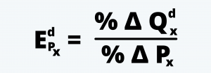
a.  The own-price elasticity of demand is the relative responsiveness of quantity demanded to change in commodity price; in other words, price elasticity is the proportional change in quantity demanded divided by the proportional change in price.

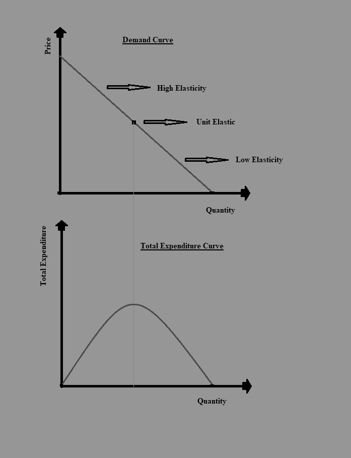
b.  Mathematically it can be presented through the following equation:

We can elaborate the numerator and denominator to write the equation as follows:

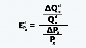
Or, we can simplify the above equation to write the elasticity of demand as follows:

c.  In the above demand function, i.e. Q_D = 303 – 0.4P; -0.4 represents the price elasticity of demand.

d.  For all negatively sloped, linear demand curves, the elasticity of demand varies depending on the point in the curve, where it is calculated.

e.  For example, for the above demand curve, the schedule of price and quantity demanded is as follows:

The slope of the curve or the term  ∆Q^d_x / ∆P_X in the equation of price elasticity of demand is “-0.4”.

Using this slope of the curve we can calculate the price elasticity of demand at each point by multiplying the curve by “P/Q” at the respective point.
Thus, the price elasticity of demand at each point would be:

f.  In the above schedule, point B is a relatively elastic point. This is because the elasticity of demand here is very high. A percentage change in the price of tea would change the quantity by a very high amount. Whereas, point G is a highly inelastic point.
If we have a price of $ 378.79 the quantity demanded would be 151.48. At this point, the price elasticity of demand is a negative 1. That is any change in price would bring the equivalent change in the quantity demanded. This point is called the unit-elastic point.
Thus, a commodity demand is elastic or inelastic accordingly as the coefficient of price elasticity is greater than or less than unity. If the coefficient is exactly one, the demand curve is said to have unitary price elasticity.

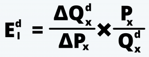
g.  This brings us to the concept of ‘perfectly elastic and ‘perfectly inelastic demand curves.

h.  A perfectly-elastic demand curve is a horizontal straight line. It represents the direct relation of the demand to a particular price, at which the demand is infinite. The perfectly elastic demand curve is as follows:

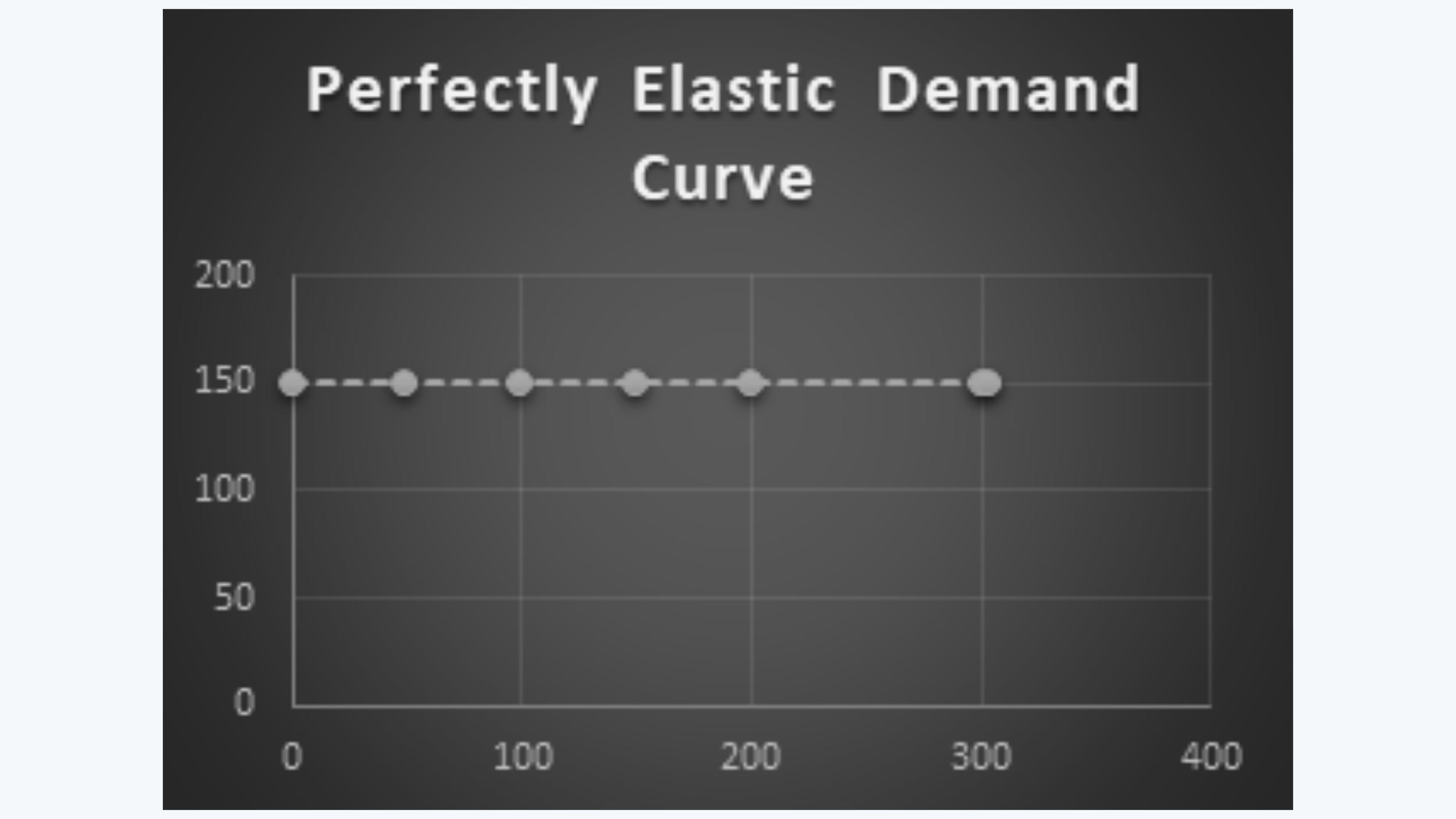
i.  A perfectly inelastic demand curve is a vertical straight line. It represents no relation of the demand to any price; the quantity demanded remains the same at all the prices. The perfectly inelastic demand curve is as follows:

1.5.           Factors that Affects Demand Elasticity

a.  Availability of Substitutes:

Substitutes are the goods or services that can be used instead of the goods and services in question.

The availability of substitutes increases the price elasticity of demand. For example, say there is a product such as a smartphone, having many substitutes available. If there is a small increase in the price of our product the demand will fall significantly because people will find an alternative to our product and substitute the same with that product. Thus, there would be a huge price elasticity of our product.

b.  A portion of Total Budget:

Higher the cost of the product, making it a part of a large share of the total budget of the consumer, higher would be its price elasticity.

For example, consider two products cars and milk. An increase in the price of the car by 20% would affect its demand more than the increase of 20% in the price of milk affecting the demand for milk.  Thus the car has higher price elasticity than the milk.

c.  Time Horizon:

The higher the time horizon of holding the product, the higher would be its price elasticity. This is mainly because, in the longer horizon, the consumer tries to find an alternative to the commodity. Thus, its price has a huge impact on the elasticity of the good.

d.  Discretionary Goods Vs. Non-Discretionary Goods:

Discretionary goods are goods that are optional in nature. Whereas, non-discretionary goods are goods that are a necessity for the consumer.

1.6.           Elasticity of Demand & Total Expenditure

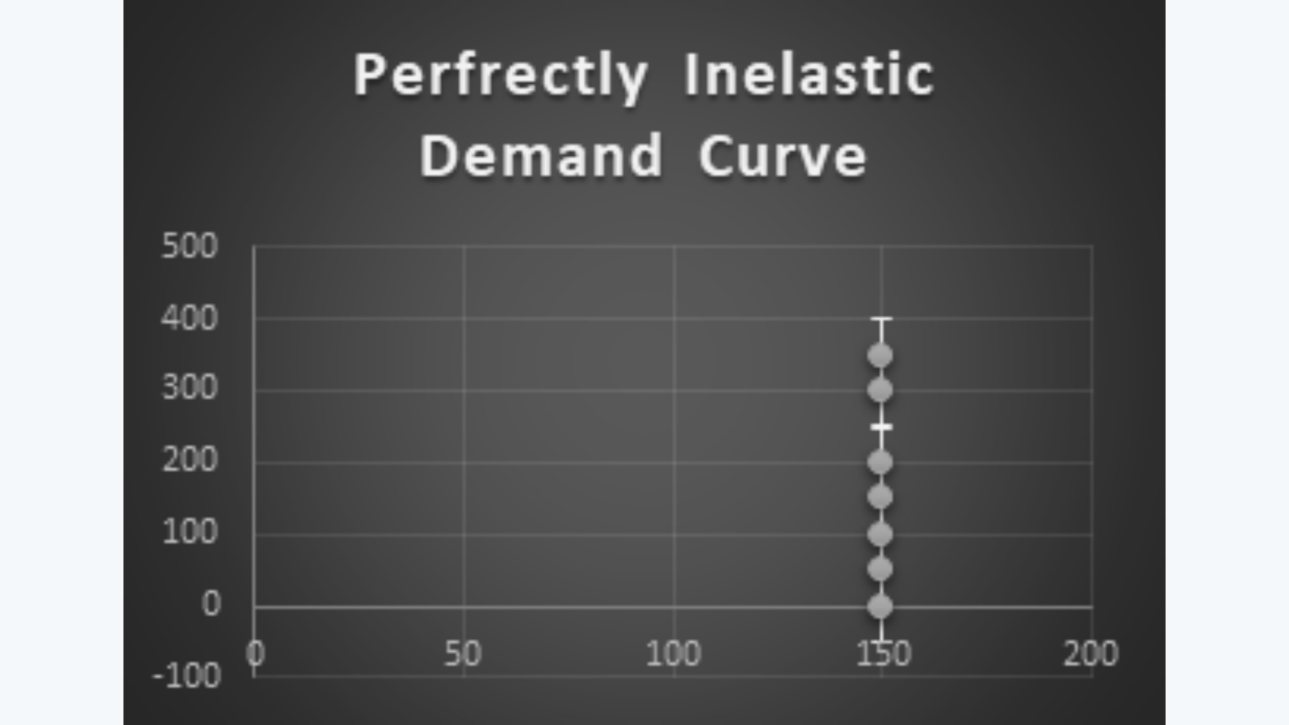
Consider the following figure:

In the above diagram, the first graph shows the demand curve, with different levels of elasticity on it. And the second graph shows the graph for total expenditure.

a.  In the first graph, the upper portion of the demand curve when the prices are high and the demand is still low has a high elasticity. At this level, the total expenditure is also rising.

b.  Somewhere in the middle of the demand curve, there is a point where the demand curve is unit elastic. It is the point where a change in the price would bring about the same percentage change in the quantity demanded. The total expenditure on the purchase of the commodity (i.e. the price multiplied by the quantity) is maximum at this point. That is, the total expenditure keeps rising up to this point, where the demand curve is unit elastic.

c.  In the lower portion of the demand curve, after the point where the demand curve is unit elastic, the elasticity of the demand is also relatively low. And, after this point, the total expenditure of the consumer also starts decreasing.

1.7.           Income Elasticity of Demand

a.  The income elasticity of demand is defined as a percentage change in the number of goods demanded, as a result of the percentage change in the level of income of the consumer.

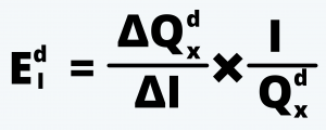
b.  It can be written in the form of an equation as follows:

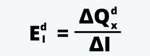
Or, we can simplify the above equation as follows:

c.  For the normal goods, the income elasticity of demand is positive, i.e. as the income of the consumer increases the demand for the goods also increases, and vice-a-versa.

d.  For the inferior goods, on the other hand, the income elasticity is negative, i.e. the demand for the goods goes down with an increase in the income level of the consumer. This is mainly because the consumer substitutes the inferior goods with the superior goods with an increase in the income levels.

1.8.           Cross Elasticity of Demand

a.  The cross elasticity of demand is the degree of responsiveness of the demand for the good to the price of other goods, everything else being constant.

b.  The price of goods that affect the prices of the goods in question is those that have a connection (either direct or indirect), with them. For example, the price of goods such as complementary goods, substitute goods, etc. affects the price of the goods.

c.  The cross elasticity of a substitute good is positive, i.e. as the price of the substitute goes up, the demand for the commodity also increases, and vice-a-versa.

d.  The cross-price elasticity of a complementary good is always negative, i.e. as the price of the complementary goods goes up, the demand for the commodity falls.

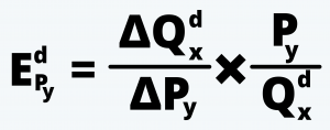
e.  Suppose we have to find the cross elasticity of a good ‘x’s in terms of the price of good ‘y’; the equation for finding the same is:

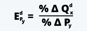
Or, we can simplify the equation as follows:

1.9.           Substitution & Income Effect

a.  As discussed above, according to the law of demand, a decrease in price results in an increase in quantity demanded. This increase in demanded quantity could be a result of two forces, i.e. income effect and substitution effect.

b.  When the consumer substitutes the goods in question with other goods because it has become comparatively cheaper, it is called the substitution effect.

c.  Whereas, when the consumer starts consuming more of the goods whose prices have fallen because their real income has increased, it is called the income effect. (It should be noted that, due to a decrease in the prices of the goods, the consumer can buy more of them, hence there is an increase in their purchasing power or the real income, despite the nominal income remaining the same.)

d.  For normal goods, with a decrease in the price of the goods, there is an increase in quantity due to both substitution effect and income effect (resulting from an increase in real income).

e.  For the inferior goods, a decrease in price would result in an increase in quantity demanded (as they still can purchase more quantity of the good. But due to the income effect, there is an increase in real income thus the consumer is more likely to shift over from inferior to better quality goods.

1.10.        Exceptions to Law of Demand

1.10.1.    Giffen Goods

a.  Giffen goods are named after Scottish economist, Sir Robert Giffen, who first observed the paradox of Giffen goods.

b.  These are the goods for which the income effect dominates over the substitution effect.

c.  For normal goods as the price of the goods decrease, there is a decrease in the quantity demanded of the goods, as people either substitute them for other goods or simply reduce the appetite for those goods.

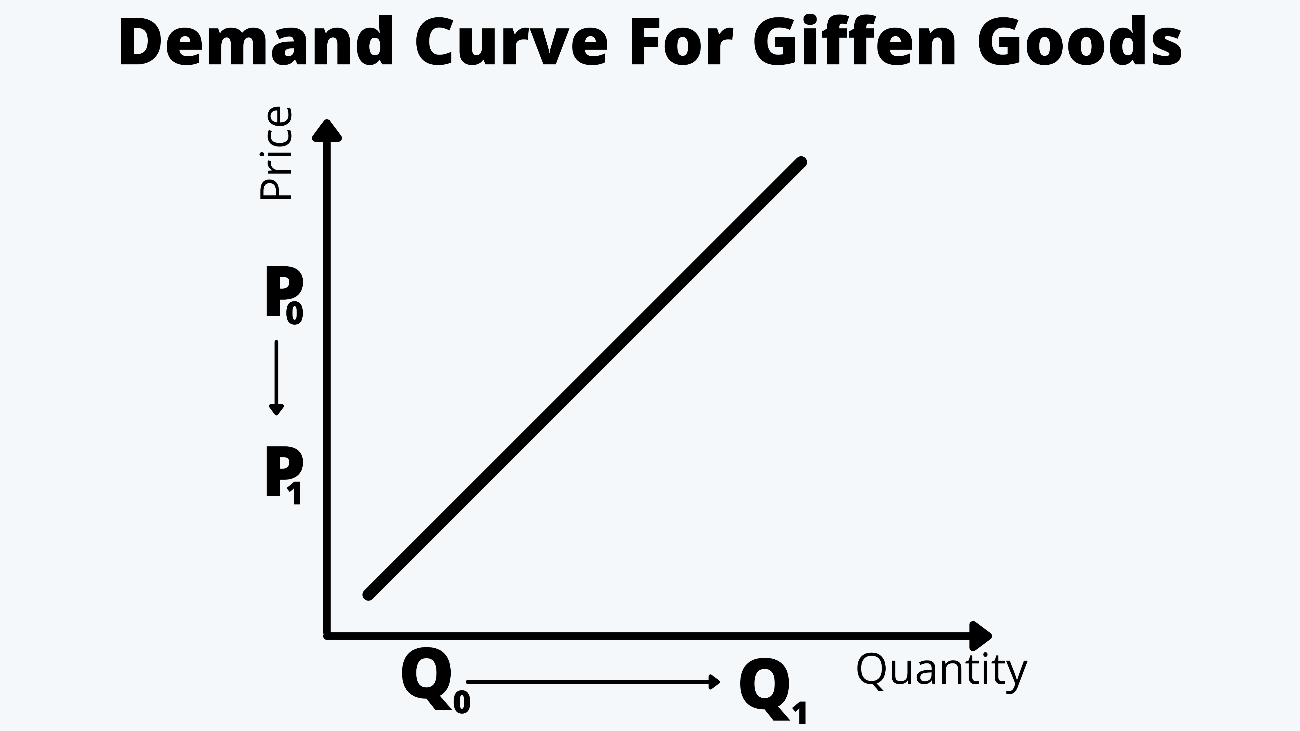
d.  But, in the case of some goods, such as inferior goods, the income effect overtakes the substitution effect. And, due to an increase in the real income, the consumers reduce the consumption of these goods and replace them with better quality or more superior goods. Therefore, in contrast to the law of demand, there is a decrease in the quantity demanded, with a decrease in the price of the goods.

e.  The slope of the demand curve is thus positively sloping, as follows:

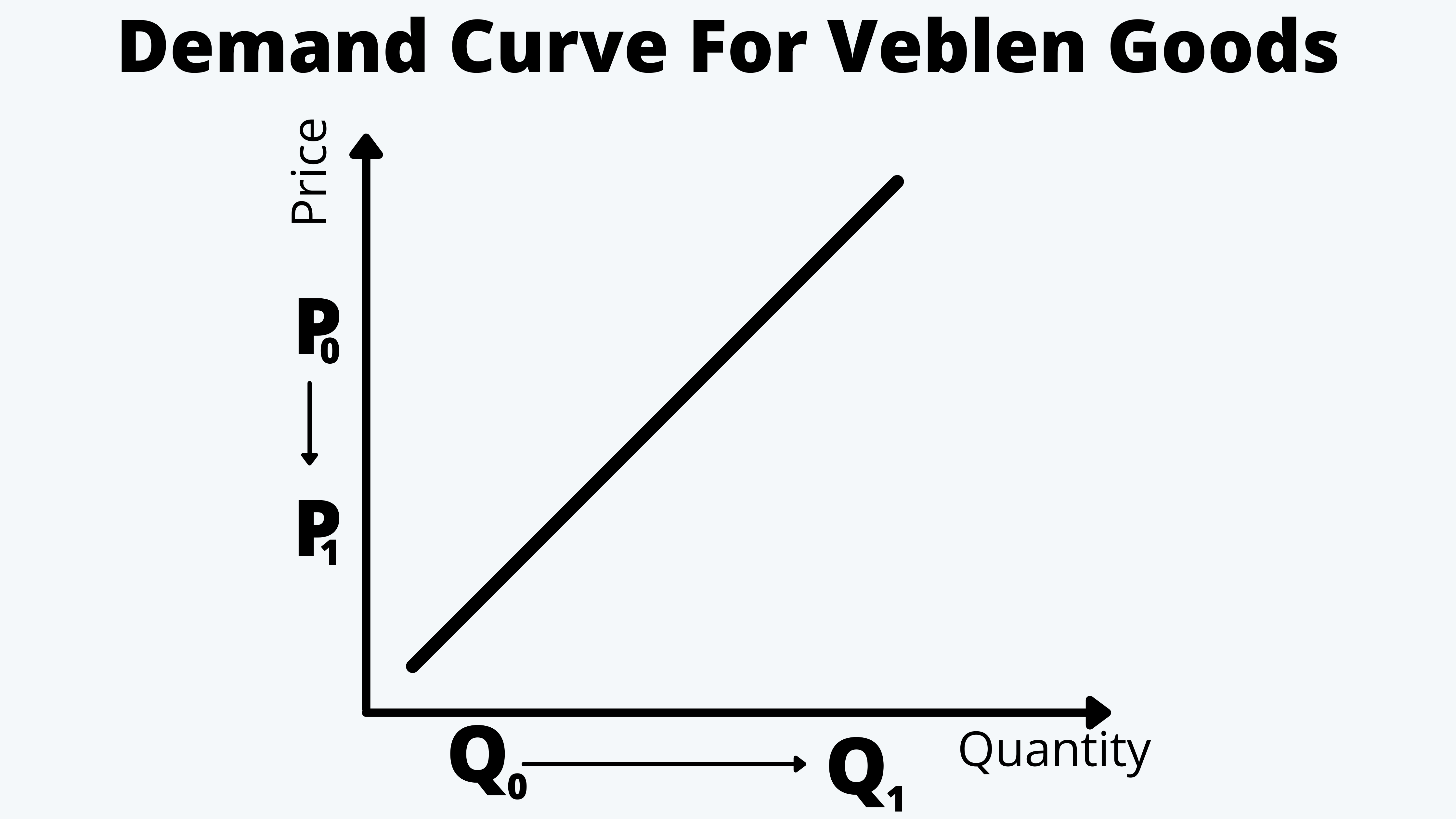
1.10.2.    Veblen Goods

a.  Veblen goods are those goods that derive their value from their high price.

b.  For example, the luxury goods such as jewelry, their demand increases with an increase in their price, as their possession becomes even dearer to the consumer.

c.  Thus, the Veblen goods also have a positively sloping demand curve like the Giffen goods.