a. In this section, we aim to look at attaining the macroeconomic equilibrium through the IS-LM
b. The equilibrium occurs when there is a demand and supply equilibrium in all the markets.
c. The demand side can be bifurcated into two goods market and money market (or assets market).
This bifurcation defines the willingness of the consumers (i.e. households and firms) in the economy to hold the money balances versus spend the same in the goods market.
d. The supply side is defined by the labor markets.
e. An economy is said to be in equilibrium when all the three markets (i.e. goods market, money market, and labor market) are in equilibrium.
i. In the goods market, we discuss a relationship between interest rates and output. This gives us the IS Curve (i.e. Investment-Savings curve).
ii. In the money market also, we discuss the relationship between interest rates and output. However, here we discuss the LM Curve (i.e. Liquidity-Money curve), which is at a given price level.
iii. In the labor market, we obtain the aggregate supply curve by working on the relationship between the output and the price.
iv. Through the IS and LM curves, we get the equilibrium in the goods market as well as the money market. We add them together to get the aggregate demand curve.
v. The aggregate demand curve so obtained is equated with the aggregate supply curve to find the equilibrium in the economy as a whole.
1.1. Aggregate Demand Curve
a. The aggregate demand curve represents the number of goods and services that households, businesses, government, and foreign customers want to buy at any given level of prices.
b. It is derived from the IS-LM curve model.
c. Through the IS-LM model, we try to identify the determinants of national income for a given price level. This also gives us an insight into what are the factors that can induce growth in output at particular price levels.
d. The IS curve gives us details about the equilibrium conditions in markets for goods and services. The LM curve, on the other hand, gives us details about the equilibrium conditions, i.e. demand and supply in the money market.
e. The interest rates influence the level of output in both IS and LM curves, And the interaction between goods and money markets at the given interest rates determines the level of national income.
1.1.1. IS Curve
a. The IS curve is obtained by equating the aggregate income with the aggregate expenditure. This results in the investment–savings (IS) curve, which is the relationship between savings less investment (S – I) and income, Y.
b. The IS curve represents the demand for money from the goods market.
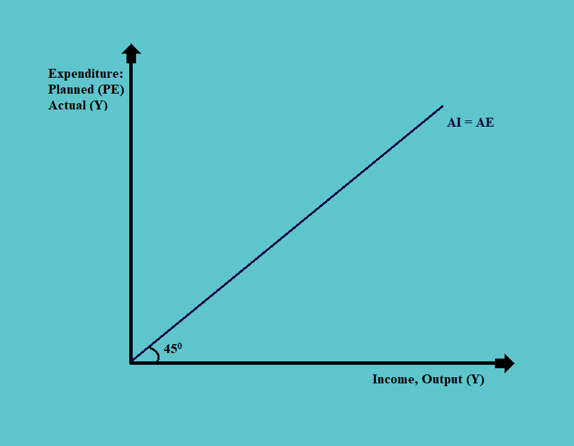
c. To understand the IS curve, we need to understand the difference between the actual and planned expenditure, as the IS curve is the investment-savings curve that represents an equilibrium between planned expenditures and income.
d. The actual consumption is the total value of goods and services consumed in the economy. This consumption is matched with the actual expenditure to find the equilibrium in the economy.
If we plot the points of equilibrium, where the actual expenditure equals the actual income, we get an upward-sloping line of an angle of 450. Thus, the slope of this line is 1.
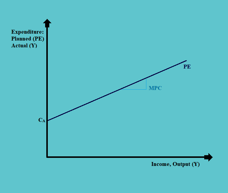
e. For the planned expenditure:
i. There is a certain level of expenditures that need to be incurred regardless of the income. Such minimum expenditure is called the autonomous expenditure (CA).
This expenditure is incurred, whether there is an income or not.
ii. As the income increases, the consumption level also increases. But all the income earned is not consumed; some is saved or invested as well.
The amount of consumption that takes place is equal to the marginal propensity to consume.
iii. If we plot this expenditure on a graph, we get an upward-sloping graph, starting at the level of autonomous expenditure, with a slope of less than 1, equal to the marginal propensity to consume.
f. The planned expenditure and the actual expenditure can be drawn together on a single graph as follows:
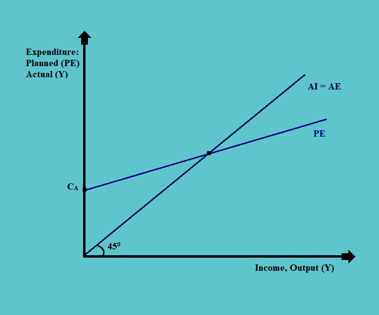
i. The equilibrium in the goods market occurs at the point of intersection of the actual expenditure and the planned expenditure curve.
ii. If the level of output is to the left of this point of equilibrium, the consumption is more than the production. Therefore, the inventories are drawn down at this level of output.
In such situations, the firms in the economy would try and increase the production and output to match the level of consumption. Thus, the output would move towards the equilibrium level.
iii. If the level of output is to the right of this point of equilibrium, the consumption is less than the production. Therefore, the inventories are built up at this level of output.
In such situations, the firms in the economy would try and reduce the production and output to match the propensity to consume. Thus, the output would again move towards the equilibrium level.
iv. Thus, there are always stabilizers in an economy that works towards bringing the level of output to equilibrium level in the goods market.
g. Now, as discussed, the IS curve can be obtained by balancing the aggregate income and aggregate expenditure. This can be done as follows:
i. As discussed, the aggregate expenditure in an economy equals consumption, investment, government spending, and net exports. That is:
AE = C + I + G + (X – M)
ii. And, the aggregate income in the economy equals the consumption, savings, plus taxes of both households and businesses. That is:
AI = C + S + T
iii. And the equilibrium point in the economy occurs when the aggregate expenditure in the economy equals the aggregate income. That is:
C + I + G + (X – M) = C + S + T
iv. Now, if we isolate S on one side we get:
S = C + I + G + (X – M) – C – T
or,
S = I + (G – T) + (X – M)
v. We can interpret the above equation by saying that ‘savings are used for three purposes, i.e. investment spending, government spending, and claims against foreigners’.
vi. The savings are, therefore, an outcome of the decision of households, firms, government, and
Therefore, the factor that determines the decisions of households, firms, governments, and foreigners also determine the aggregate income and expenditures.
h. As discussed, for the IS curve, we need to balance the aggregate income with the aggregate expenditure. Also,
AE = C + I + G + (X – M)
And, the graph on which we plot the IS curve has an output (Y) on the x-axis and rate of interest (r) on the y-axis. Thus, aggregate expenditure along with each of its components is a function of Y and r. Therefore,
i. Consumption is an increasing function of disposable income (i.e. Yd). Thus, the more disposable income; the more is the level of consumption. The disposable income is total income minus the taxes (i.e. Yd = Y – t).
Also, it is a decreasing function of interest rate (i.e. r). This is mainly because, as the interest rates go up, the marginal propensity to consume goes down. People tend to save more in such situations.
We can thus say,
C = C (Y – t, r)
Thus, an increase in income or a decrease in taxes or interest rates will increase the aggregate expenditure. Also, the larger the marginal propensity to consume, the greater will be the impact.
ii. The investment (i.e. I) is a function of interest rates and aggregate expenditure. This is mainly because; the interest rates affect the cost of financing and the aggregate expenditure affects the expected profitability of new investments. Thus,
I = I (r, Y)
In the above equation, therefore, the investment is an increasing function of output and a decreasing function of real interest rates.
iii. The government expenditure (G) is treated as an exogenous item. This means that the government budget is fixed and it does not change with the level of income. We express the government deficit as follows:
G – T = Ḡ – t(Y)
The above equation, Ḡ indicates that the government budget is fixed whereas taxes are an increasing function of the level of income.
iv. For the net exports, the exports are also treated as exogenous items because they depend upon the demands from the rest of the world. However, the imports are an increasing function of the levels of income (i.e. Y).
i. We can explain the IS curve with the help of an example.
As we know that:
Y = C + I + G + (X – M)
And we are given that:
i. C = 2000+ 0.5 (Y – T); (which is an increasing function of Y)
ii. I = 400 + 0.2 Y – 30 r; (which is an increasing function of income, and a decreasing function of interest rate)
iii. G = 1500; (it is exogenous and we are given a value for it)
iv. X – M = 1000 – 0.10 Y; (thus our imports are a decreasing function of the level of income)
v. T = -200 + 0.3 Y; (the autonomous part of the taxes is negative because the government has to make payment with regards to the transfer payments, whether there is income or not).
We substitute the values of all of the above in the equation of Y to get:
Y = 2000 + 0.7 (Y – T) + 400 + 0.2Y – 30r + 1500 + 1000 – 0.10Y
or,
Y = 2000 + 0.7 (Y + 200 – 0.30Y) + 400 + 0.2Y – 30r + 1500 + 1000 – 0.10Y
If we solve the above equation we get Y as a function of r, i.e.:
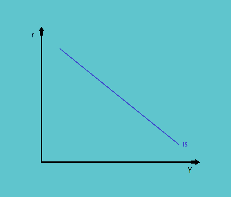
Y = 12292.69 – 73.2r
The above equation, if drawn on a graph will result in a downward-sloping curve with an intercept of 12,292.69 and a slope of 73.2. Thus, the IS curve will look like this
1.1.2. LM Curve
a. The LM curve stands for the liquidity-money curve. All the points on the curve show the combination of interest rates and income where the demand for money equals its supply.
b. Some of the terminologies used while discussing the supply-side of the LM curve is:
i. M = It stands for the supply of money
ii. P = It represents the price level
iii. (M/P)s = Supply of real money
We assume here that there is a fixed nominal supply, thus ‘M’ in the numerator is fixed. Also, in the short run, we keep the value of ‘P’ fixed too. In the long run, however, in order to derive the aggregate demand curve, we change the value of ‘P’ while keeping the ‘M’ constant.
Therefore, in the short run, we have:

where both ‘M’ and ‘P’ are considered as exogenous variables.
We can, therefore, plot the demand and supply of the money in short-run as follows:
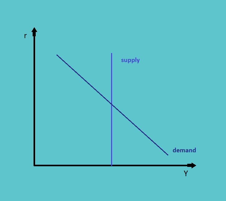
The supply curve is thus one straight line, as the supply of money is exogenous.
c. While discussing the demand-side in the money markets, it is extremely important to discuss liquidity.
It is the amount of money that the market participants are willing to hold. In tough times, people require more liquidity and vice-versa.
There are three main reasons for which there is a need for liquidity; they are:
i. Transactional Needs: The market participants need money for making purchases in the market for consumption and other requirements.
ii. Precautionary Needs: To be on the safer side, the market participants tend to save more money than what is needed for consumption, which may be required in the case of an emergency.
iii. Speculative Needs: The participants may come across sudden earning opportunities, which may be speculative in nature. People need to keep money in their hands to reap profits in such situations as well.
As the real interest rates rise, the opportunity cost of holding money balances or liquidity increases.
Therefore,
|
(M/P)d decreases when r increases |
This is the reason, why we have a downward-sloping demand curve in the money market. And, liquidity is a decreasing function of the real interest rate. That is,
| (M/P)d = L(r) |
d. Using the demand and supply curve for the money, as derived above, we can calculate the LM curve as follows:
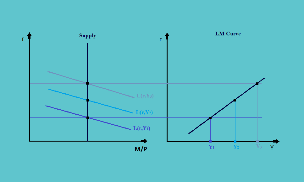
In the above figure, the left graph shows the supply and demand situation in the money market.
i. We begin with the level of real supply of money and the interest rate in the market which gives the equilibrium at the point where the demand curve (i.e. L(r, Y1)) intersects the supply curve.
ii. Now suppose there is an increase in the level of income. This will result in a shift upwards in the demand curve (assuming other things remain constant). This will result in another level of equilibrium. Similarly, a further rise in the level of income will result in another level of equilibrium.
iii. The graph on the right has income level on the x-axis and interest rates on the y-axis.
iv. If we join the level of interest rates at the equilibrium level in the money market (from the left graph) with the level of income (in the right one), we get the combinations of interest rates and level of income at which the money market is in equilibrium. This downward-sloping curve is called the LM curve.
1.1.3. Derivation of Aggregate Demand Curve
a. For the derivation of the aggregate demand curve from the IS-LM framework, we keep the supply of money and change the prices, unlike the change in the level of income, as done previously. Consider the following figure:
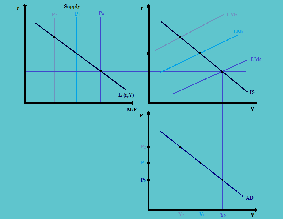
b. The graph on the upper left-hand corner represents the supply and demand in the money markets. The one on the upper right-hand side represents the IS and LM curve. In the graph at the bottom, we finally derive the aggregate demand curve.
c. When there is an increase in the prices in the money market, the demand for the money is unaffected. However, due to inflation, there is a fall in the real supply of money. This results in the supply curve shifting inwards.
Thus, when there is an increase in the prices from P0 to P1, and finally to P2; there is a respective shift in the supply curve inwards.
d. The shift in the supply curve results in disequilibrium in the IS-LM graph. In order to have the equilibrium back, there should be a shift inwards in the LM curve.
Thus, a new equilibrium is attained at a lower level of income at the decreased price levels.
e. If we plot the changes in prices and the corresponding equilibrium level of income, as in the bottom graph, we get the aggregate demand curve in the markets.
f. Thus, the aggregate demand curve is a combination of equilibrium income levels at different levels of prices.
g. One thing that needs to be noted is that any changes in the IS or the LM curve will be reflected in aggregate demand (AD) through the effect on the price level.
i. Fiscal policy will shift the IS curve (e.g., expansionary fiscal policy shifts the IS curve to the right).
ii. Monetary policy will shift the LM curve (e.g., increased money supply shifts the LM curve to the right, as shown in the graph on this slide).
h. Thus, in order to make changes in the aggregate demand in the economy, one should make amendments to the fiscal and monetary policies.
1.2. Aggregate Supply Curve
a. The aggregate supply (AS) curve represents the level of domestic output that companies produce at each price.
b. Before we discuss the aggregate supply curve, we need to understand the concept of ‘sticky wages’. In the short run, the wages are fixed because it is difficult to adjust the wages in a very short frequency. Also, the workforce resists any downwards movements in wages. In the long run, however, the wages can adjust. Thus, we say that wages are sticky in the short run.
c. Since wages have a direct impact on the amount of supply, we have three different types of supply curves in different time horizons.
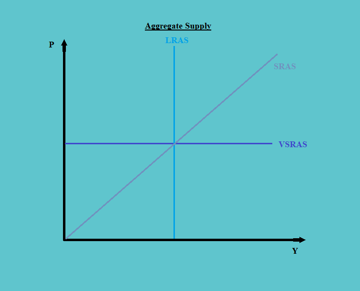
i. In the very short run, the aggregate supply curve is a horizontal line as the supply is not responsive to the price changes. This is mainly because; in the very short run the companies can increase or decrease the supply, as long as the profits are more than the variable costs.
ii. In the short run, the supply curve becomes upward-sloping, as the output becomes more responsive to the price changes.
In the short run, more costs become variable with time. As time passes, short-term contracts roll over and reflect the changes in wages and input prices.
Thus, in the short run, the output increases with the increase in prices and vice-versa.
iii. In the long run, all variable costs, including the wages can fully adjust to the price changes. Thus, in the long run, the supply position is determined by the potential output.
All the variables, such as labor and capital, become fixed in the long run. Thus the supply becomes exogenous, and the supply curve becomes a vertical straight line.
1.3. Shifts in Aggregate Demand & Aggregate Supply Curve
1.3.1. Shifts in Aggregate Demand curve
As seen above, the aggregate demand curve is a negatively sloped downward-slopping curve. It may shift inwards, towards the left, or may shift outwards towards the right, as seen in the figure below:
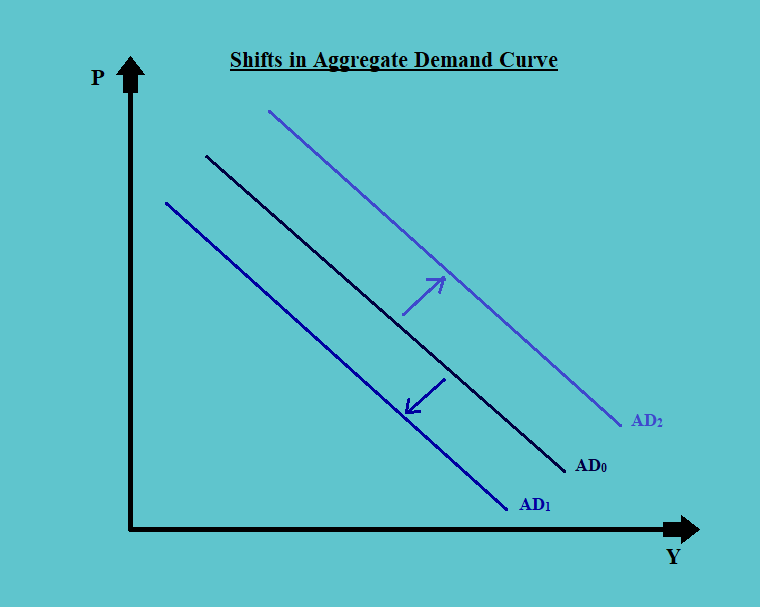
In the above figure, a shift from AD0 to AD1 shows a decrease in demand at any given price levels; whereas, a shift from AD0 to AD2 shows an increase in demand at any given price levels.
There may be many reasons for such shifts; some of the important reasons are:
a. Household Wealth: Household wealth includes all the assets held by the households including both real as well as financial. It affects the aggregate demand as follows:
i. An increase in the household wealth will increase the current level of consumption and decrease the savings, thus shifting the aggregate demand outwards, toward the right.
ii. A decrease in the household wealth will decrease the current level of consumption and increase the savings, thus shifting the aggregate demand inwards, toward the left.
b. Consumer and Business Expectations: This refers to the confidence of the market participants in the market conditions. It affects the aggregate demand as follows:
i. An increase in the confidence levels will increase the marginal propensity to consume of the consumers and marginal propensity to invest of the investors. This will result in an outward shift in the aggregate demand curve towards the right.
ii. A decrease in the expectations will decrease the marginal propensity to consume of the consumers and marginal propensity to invest of the investors. This will result in an inward shift in the aggregate demand curve towards the left.
c. Capacity Utilization: Capacity utilization refers to the use of investment towards production. When the investment levels increase, there is a corresponding increase in the aggregate demand; resulting in an outward shift in the demand curve and vice-versa.
d. Fiscal Policy: The fiscal policies comprise of two main components, i.e. government taxes and spending. It affects the aggregate demand as follows:
i. An increase in government spending and a decrease in the levels of taxes increase the aggregate demand, making the aggregate demand shift outwards.
ii. A decrease in government spending or an increase in the tax collection, on the other hand, decreases the aggregate demand, making the aggregate demand shift leftwards.
e. Monetary Policy: As a part of the monetary policy, the government may make changes to the bank reserves, reserve requirements, and target interest rates, etc. These changes affect the aggregate demand as follows:
i. A decrease in the bank reserves or an increase in the reserve requirements and target interest rates reduces the real supply of money, thus reducing the investment and consumption spending. This results in a decrease in the aggregate demand, resulting in an inward shift in the demand curve.
ii. An increase in the bank reserves or a decrease in the reserve requirements and target interest rates increases the real supply of money, thus increasing the investment and consumption spending. This results in an increase in the aggregate demand, resulting in an outward shift in the demand curve.
f. Exchange Rate: The exchange rate affects both the exports and the imports, thus affecting the aggregate demand as well.
i. An increase in the foreign exchange rate decreases the levels of exports and increases the level of imports, thus reducing the aggregate demand.
ii. A decrease in the foreign exchange rate increases the levels of exports and decreases the level of imports, thus increasing the aggregate demand.
g. Global Growth: A decrease in global growth decreases the level of exports and thereby reducing the aggregate demand, shifting the aggregate demand curve to the left, and vice-versa.
1.3.2. Shifts in Short-Run Aggregate Supply Curve
As discussed, in the very short-run and long-run, the supply curve is fixed horizontal and vertical line respectively. However, in the short run, the supply curves do tend to shift. The factors that change the cost of production or expected profit margin, results in a shift in the supply curve.
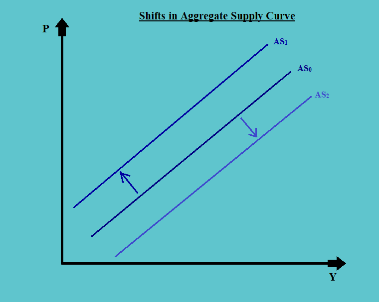
When there is an increase in the total output at any given price level, there is an outward shift in the aggregate supply curve (like from AS0 to AS2 in the above figure). And when there is a decrease in the total output at any given price level, there is an inward shift in the aggregate supply curve (like from AS0 to AS1 in the above figure).
Some of the most important causes of the shift in the short-run aggregate supply curve are:
a. Shifts in Long-Run Aggregate Supply Curve: Since both long-run and short-run aggregate supply curve reflects the same underlying levels of technology, a leftward shift in the LRAS will shift the SRAS towards the left and a rightward shift in the LRAS will shift the SRAS towards the right.
b. Changes in Nominal Wages: An increase in the wages decreases the level of production and vice-versa, in the short run. In the long run, however, there is no impact of the changes in wages on the changes in production.
Therefore, as a result of a decrease in wages, the aggregate supply curve moves inwards, and vice-versa.
c. Changes in Input Prices: Like wages also an increase in the input prices results in a decrease in production; thus shifting the short-run aggregate supply curve inwards; and vice-versa.
d. Changes in Expectation of Future Prices: If there is an expectation of lower prices in the future, the producers will tend to produce less (as the produce will fetch less money and lowering the supply could possibly act as price corrector), and vice-versa. Thus, the lower expectation of future prices will shift the short-run aggregate supply curve inwards and a higher price expectation will shift the aggregate supply curve outwards.
e. Changes in Business Taxes and Subsidies: An increase in taxes and a decrease in subsidies shift the short-run aggregate supply curve inwards and a decrease in taxes and an increase in subsidies shift the aggregate supply curve outwards.
f. Changes in Exchange Rates: An increase in the foreign exchange rates makes the exports cheaper and the imports costlier. Therefore, the level of exports increases and imports decreases. This results in an increase in the level of output to facilitate the increased levels of exports and reduced imports, thus shifting the aggregate supply curve outside. The opposite is true for a decrease in the foreign exchange rates.
1.3.3. Shift in Long-Run Aggregate Supply Curve
Any factor that changes the resource base in an economy can shift the long-run aggregate supply curve.
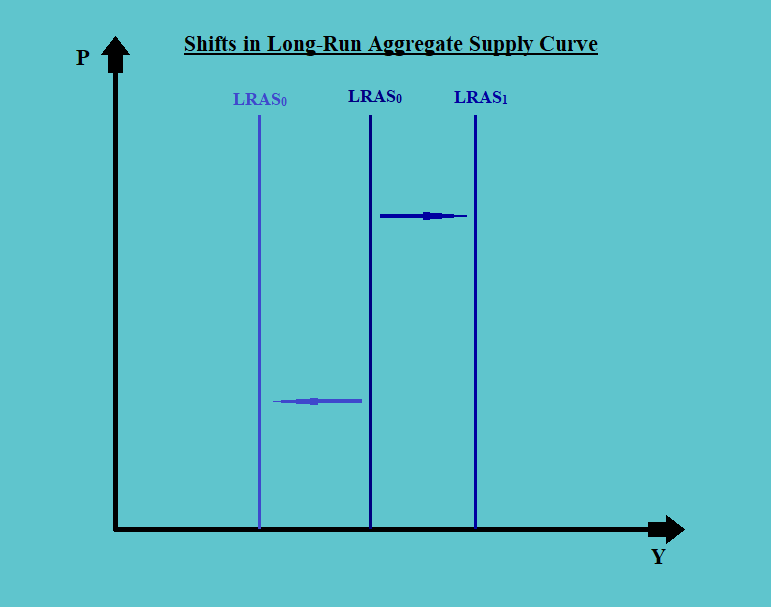
A shift outwards from LRAS0 to LRAS1 represents increased potential output, whereas, a shift inwards from LRAS0 to LRAS2 represents the decreased potential output.
Some of the factors that affect the movements in the long-run aggregate supply curve are:
a. Supply of Labor: An increase in factors such as population, participation rate, net immigration, etc. increases the supply of labor. This results in an increase in total production, leading to an increase in the aggregate supply. This, in turn, results in a shift of LRAS outwards towards the right. The opposite is true for the decrease in such factors.
b. Supply of Physical Factors: An increase in the supply of physical factors increases the total production, resulting in the shift of the aggregate supply curve outwards; and vice-versa for a decrease in such supply.
c. Supply of Human Capital: An increase in the supply of human capital resulting due to an increase in quality of labor increases the total production, resulting in the shift of aggregate supply curve outwards; and vice-versa for a decrease in such supply.
d. Labor Productivity & Technology: If there is improved efficiency in the labor productivity and technology resulting in higher output per labor hour. This will lower the cost of production and increase the total output, shifting the LRAS towards the right. The opposite is true in the case of lower efficiency.
It should be noted that investment towards improvement in technology and research & development can improve labor productivity.
1.4. Equilibrium, GDP & Prices
a. Equilibrium is the price level and output at which the aggregate demand and aggregate supply curves intersect. Typically an equilibrium can be presented in the form of a graph as follows:
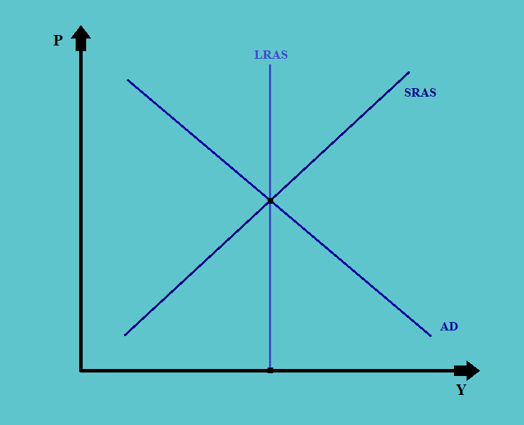
Equilibrium typically happens when the short-run aggregate supply curve intersects the aggregate demand curve over the long-run aggregate supply curve.
b. The long-run aggregate supply curve is also the long-run potential GDP. This GDP cannot be accurately estimated. However, we can estimate the long-run potential growth rate.
c. The long-run growth rate is typically rising. Thus, its graph is usually upwards sloping.
The short-run growth rate can be either above or below the long-run curve, depending on whether the economy is over-performing or under-performing in the short run.
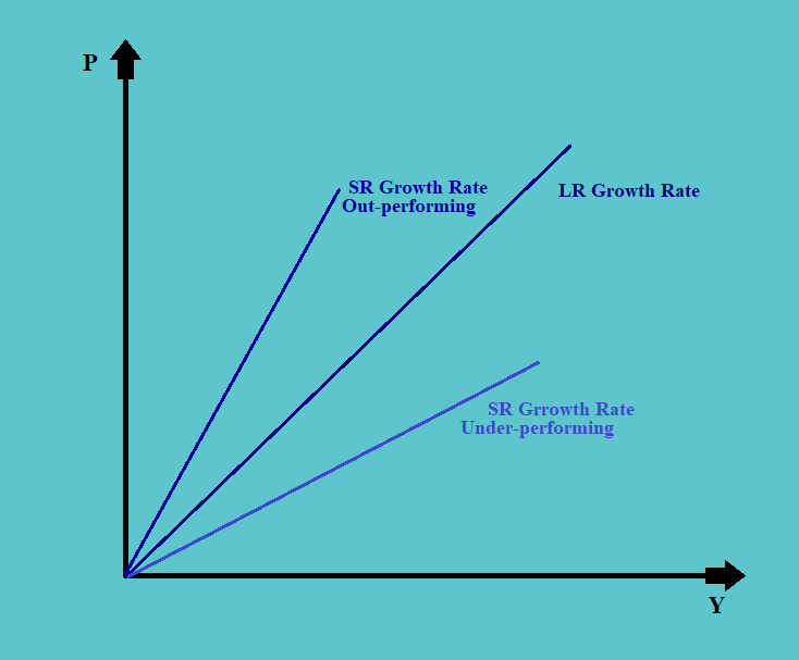
The under-performance and out-performance in the short-run in an economy result in the business cycles.
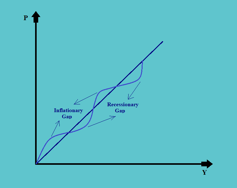
In the above figure we can see that in the short-run when the growth rate is above the long-run rate, there is an inflationary gap. And, when it is below the long-run rate, there is a recessionary gap.
d. A business cycle consists of expansion and contraction. Shifts in aggregate demand and aggregate supply determine changes in the economy.
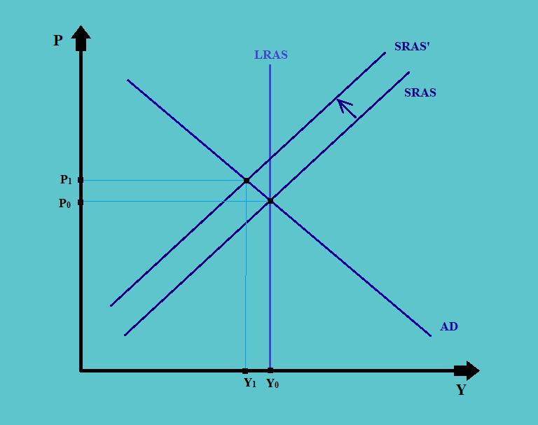
1.4.1. Recessionary Gap
a. A short-run recessionary gap exists when the economy is in a recession and equilibrium output is less than potential GDP.
b. A situation of recessionary gap generally happens when there is an inward shift in the aggregate demand curve.
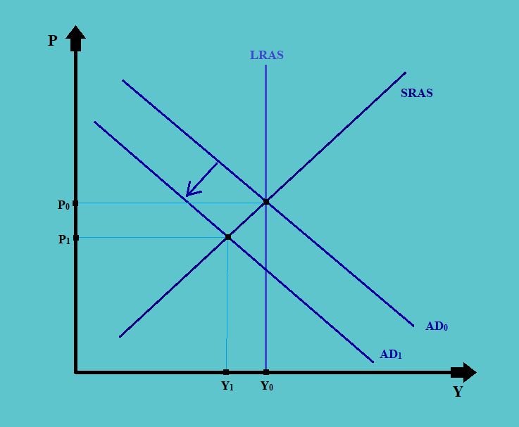
c. The inwards shift in the aggregate demand from AD0 to AD1 results in a fall in the aggregate output from Y0 to Y1, and prices from P0 to P1. This usually happens in response to certain supply contracts and an increase in unemployment, etc.
1.4.1.1. How to fix the recessionary gap?
The recessionary gap in the growth can be fixed through one of the following ways:
a. Market Auto-Correction: The market mechanism is such that it automatically corrects the short-term disturbances itself. The fall in aggregate demand will lead to lower prices, which will, in turn, induce the demand, thus correcting the fall in demand.
b. Fiscal and Monetary Intervention: The government can opt for fiscal intervention such as increased government spending and reduced taxes, or monetary interventions such as a reduced rate of interest or an increase in the nominal money supply.
1.4.1.2. Implications & Action Required for Recessionary Gap
The recessionary gap has the following implication for the economy:
a. The decrease in the levels of profit
b. The decline in commodity prices
c. Drop-in interest rates
d. Lower demand for credit or loanable funds
As an investor one can take the following actions in case of recessionary gaps:
a. Follow a ‘low-beta strategy, i.e. substitute defensive for cyclical stocks
b. Invest in quality stocks and bonds only
c. And in the bond markets lengthen the duration of the bonds
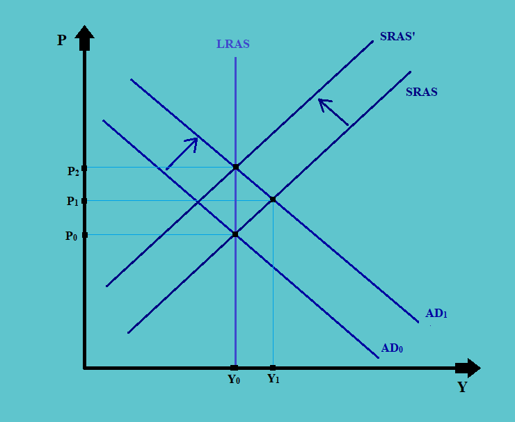
1.4.2. Inflationary Gap
a. A short-run inflationary gap exists when the economy drives GDP beyond the potential GDP. When price levels increase, short-run supply increases and the economy returns to the long-run equilibrium.
b. An inflationary gap is the exact opposite of the recessionary gap. In the case of the inflationary gap, the aggregate demand curve shifts outwards, towards the right.
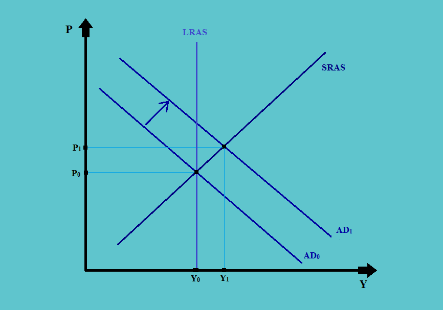
c. In such situations, the real GDP growth rate is greater than the long-run growth potential, resulting in the aggregate demand shifting from AD0 to AD1. This increases the equilibrium output and prices.
d. In the long-run, however, the free-market mechanism comes under operation and the short-run aggregate supply curve shifts inwards to SRAS’ (as a result of higher wages and raw material cost). Thus, the equilibrium output returns to Y0, but the prices increases manifold to P2.
1.4.2.1. Implications & Action Required for Inflationary Gap
The inflationary gap has the following implication for the economy:
a. The rise in levels of profits
b. A rise in commodity prices
c. Very high-interest rates
d. Building up of inflationary pressure
As an investor one can take the following actions in case of inflationary gaps:
a. Follow a “high-beta” strategy, i.e. substitute cyclical for defensive stocks
b. Increase the exposure towards commodity investment
c. And in the bond markets shorten the duration of the bonds
d. Opt for high yield rather than high-quality investment
1.4.3. Stagflation
a. Short-run stagflation occurs when there are high unemployment and increased inflation brought on by a drop in aggregate supply. The downward pressure on wages and input prices eventually brings long-run full employment.
b. In the situation of stagflation, unlike in the situation of inflation and deflation, where there was a shift in the aggregate demand curve; here there is a shift in the short-run aggregate supply curve, inwards.
In the above figure, due to the shift in the short-run aggregate supply curve from SRAS to SRAS’, there is a fall in the level of total output from Y0 to Y1 and an increase in the price levels from P0 to P1.
c. The main reason why there is an increase in the prices coupled with the fall in output is that the firms have less contribution margin to cover the fixed cost; therefore, the prices must go up to maintain the profit.
1.4.3.1. Implications of & Actions Required in Case of Stagflation
The main implications of stagflation in an economy are:
a. There is a higher rate of inflation or higher price levels
b. Stagflation also results in higher unemployment, due to decreasing output
c. Stagflation slows down the market mechanism
As an investor one can take the following actions in case of stagflation
a. For investment one should prefer the companies with higher pricing powers
b. Increase the investments in defensive stocks such as utilities
1.4.3.2. How to fix a stagflation situation?
One can fix the stagflationary situations by using one of the following policy measures:
a. Use fiscal or monetary policies to boost the aggregate demand. This will shift the aggregate demand curve outwards, to attain a new equilibrium at a higher level of output, but at a very high price.
b. Boosting the aggregate demand does increase the level of output, but it also increases the price manifold. Therefore, it is better to focus on the policies that increase the aggregate supply and brings it back to the level of SRAS.
1.5. Shifts in Both Aggregate Demand and Aggregate Supply Curves
Sometimes there is a corresponding shift in both the aggregate demand and aggregate supply curves, which does change the equilibrium level of output, but the effect on the prices of such shift is uncertain.
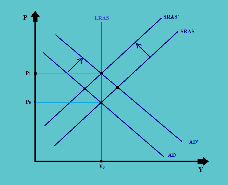
1.5.1. Right Shift in AD and AS
Consider the following figure:
a. In the above figure, there is a shift in the aggregate demand curve from AD to AD’.
b. That creates a pressure of inflationary gap, so there are market pressures that push the short-run aggregate supply curve outwards from SRAS to SRAS’.
c. Due to these shifts, the equilibrium output shifts from Y0 to Y1. However, whether there is a change in the price level or not, is uncertain.
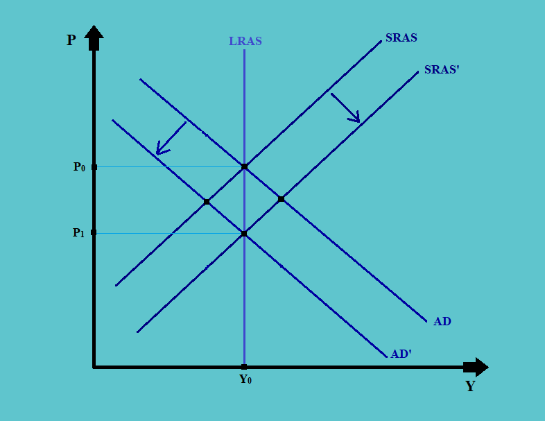
1.5.2. Left Shift in AD and AS
Consider the following figure:
a. In the above figure, there is an inward shift in the aggregate demand curve from AD to AD’.
b. At the same time, there are forces in the market shifting the aggregate supply curve also inwards, from SRAS to SRAS’. This shift may be a result of market anticipation of a fall in the aggregate demand, and a response to such a situation by the producers.
c. This results in a fall in the total output produced and consumed, but the effect on the prices is uncertain.
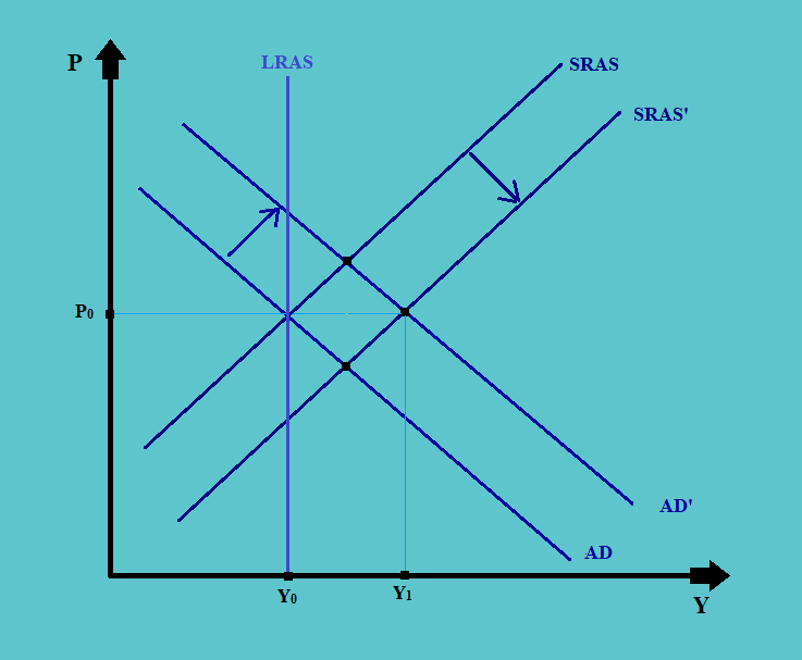
1.5.3. Right Shift in AD and Left Shift in AS
Consider the following figure:
a. In the above figure, there is an expansion in demand leading to a shift in the demand curve from AD to AD’.
b. At the same time, there may be a short-run fall in supply, shifting the short-run supply curve from SRAS to SRAS’.
c. In such a situation, there is increased demand and low supply. This increases the price manifold, from P0 to P1. Though the change to the equilibrium level of output is uncertain.
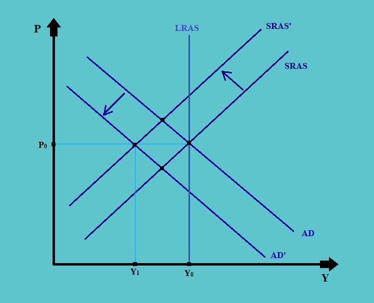
1.5.4. Left Shift in AD and Right Shift in AS
Consider the following diagram:
a. Suppose there is a fall in demand in the market. This results in the leftward shift in the aggregate demand curve from AD to AD’.
b. Also, suppose that the producer is not correct in anticipating the fall in demand, and instead, they increased the supply, shifting the aggregate supply curve rightwards from SRAS to SRAS’.
c. The situation of low demand and high supply will bring the prices really down from P0 to P1. However, the impact on the level of output is uncertain.