Present Value Models
a. The main rationale behind using this model is that the intrinsic value of a security is the present value of all the future dividends receivable from it.
b. The consumption is deferred today by the investors to have the benefits at some future point in time, and these future benefits are discounted using the expected rate of return to get its present value.
c. The simplest form of the present value model is the dividend discount model (DDM). As per this model, the value of the share is calculated as follows:
|
Where, V0 = Value of share today. Dt = Expected Dividend in the year t. r = required rate of return. |

The required rate of return used in this model is usually calculated using the CAPM or Capital Asset Pricing Model. As per CAPM, the required rate of return is calculated as follows:
|
Where, re = required rate of return rf = risk-free rate β = beta coefficient rm = market return |

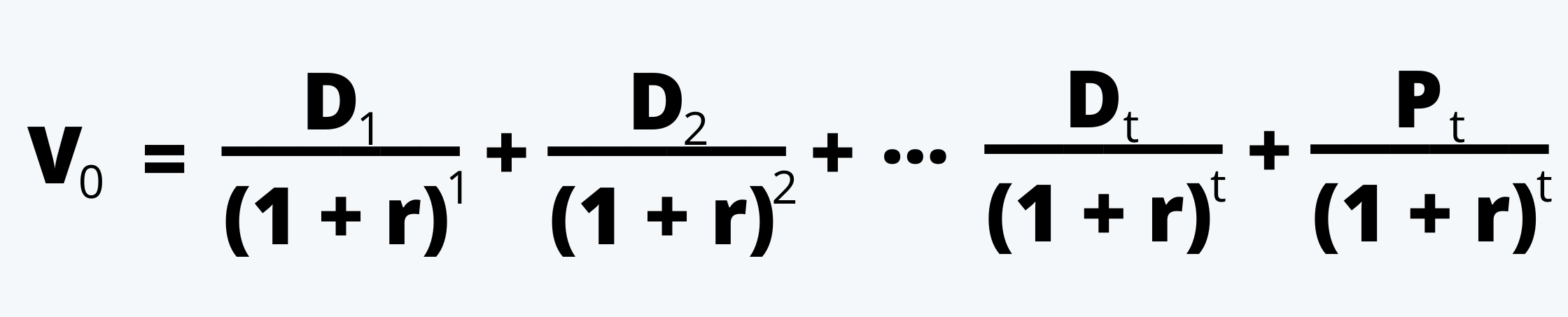
e. If there is a single holding period, i.e. the security would be held for only one period (here t=1). The securities in these cases are sold at the end of period one. The value of such securities at the beginning of the period is the discounted value of the dividend receivable one year hence plus the discounted value of the price it would fetch when it would be sold in the market. In the form of an equation it can be written as:
|
Where, Dt = Dividend at the end of period t Pt = Price at the end of period t Where t is usually 1. |

And the price of the security at the time t is:
 |
f. If there are multiple holding periods, i.e. t >1, the value of the security at the time zero is the discounted value of all the future dividends and the price it would fetch when sold. Thus the value of the security would be:
|
|
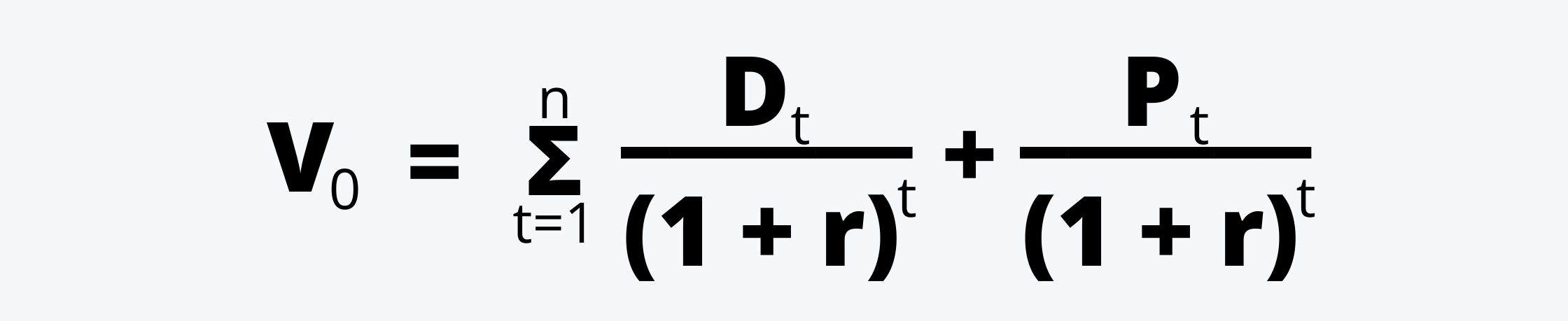
We can also write this equation as:
|
|
f. All three equations, whether of the basic model, or single-period model, or the multiple period models; all give the same value of the security. This is mainly because, in the latter two models, the price at which the security is expected to be sold is nothing but the discounted value of all the future cash flows starting at time t.
Free Cash Flow to Equity
a. This model is like the dividend discount model, discussed above; except for a significant change that free cash flow to equity replaces dividends in this model.
b. The free cash flow to equity reflects the dividend-paying capacity of the company and not the actual dividends paid. Thus, it is most useful for the non-dividend paying stocks and the companies with a high capital reinvestment opportunity.
c. The value of the firm as per this model is:
|
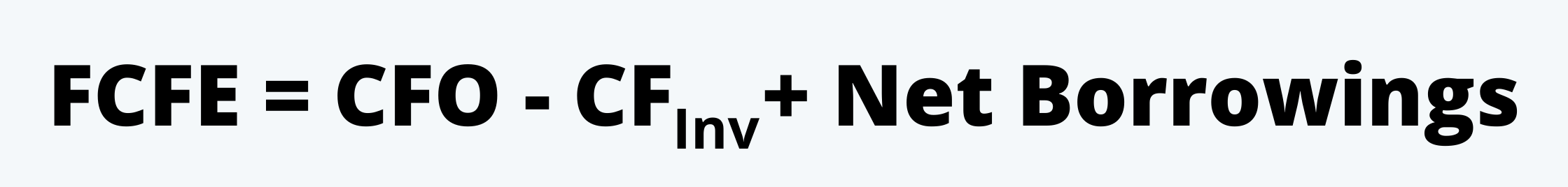
Where, CFO = Cash flow from operations CFInv = Capital Expenditure |

FCFE is nothing but free cash flow to equity, it can be calculated using the following formula:
|
Where, V0 = Value of share today. FCFEt = Free cash flow to equity in the year t. r = required rate of return. |
d. Here also the r, i.e. the risk-free rate is calculated using the CAPM as follows:
|
Where, rf = risk-free rate is the rate of return on government bond or company bond yield. β(rm– rf) = market risk premium and is subject to economic judgment. |