a.  Leverage is the use of fixed cost in the capital structure of the company. The degree of leverage is the sensitivity of net income to the change in the number of goods sold.

b.  When we talk about the impact of the degree of leverage on a company, we basically talk about two kinds of leverages, i.e. degree of operating leverage and the degree of financial leverage.

1.1.         Degree of Operating Leverage

a.  The degree of operating leverage or DOL refers to the percentage change in the operating profits as a result of a percentage change in the quantity of goods sold.

b.  DOL is calculated in different quantities. The degree is different at different levels of quantities.

c.  DOL can be calculated using the following formula:

d.  We can re-write the above equation as:

e.  We can also interpret this as contribution margin divided by the operating profit, or:

Or,

Where CM/U is the contribution margin per unit.

Example 2:

In the first example, we can calculate the DOL of both the companies in the following ways:

     i.  Using Short-cut: We can use the following formula to calculate the DOL:

DOL = Contribution Margin / Operating Profit

The DOL for company A and company B would be:

DOL_A = 90000/40000 = 2.25

DOL_B = 60000/35000 = 1.71

    ii.   Using Longer Method: We can use the following formula to calculate the DOL:

DOL = (Q × CM/U) / [(Q × CM/U) – FC]

The DOL for company A and company B would be:

DOL_A = (15000 × 6) / (15000 × 6) – 50000 = 2.25

DOL_B = (15000 × 4) / (15000 × 4) – 25000 = 1.71

Thus, in the given example, a 1% change in quantity produced and sold would bring a 2.25% and 1.17% change in the operating profit of the company.

Example 3:

If in the first example, we change the quantity of goods then there would be a different impact on the degree of operating leverage. Consider the following situations, where the quantity: a. decreases to 10,000 and increases to 20,000 (other information being the same).

Following would be the income statement under the two situations:

As calculated before, the DOL for companies A and B are 2.25 and 1.71. This means, if there are a 33.33 percent increase and decrease in the quantity of goods produced and sold, there should be DOL times the increase in operating profits.

Thus, the decrease/increase in operating profits would be:

Company A: %ΔOp.Pr. =  2.25*33.33 = 75%

Company B: %ΔOp.Pr. =  1.71*33.33 = 57.14%

The actual changes in the percentage of operating profits are:

Thus, the increase and decrease in the percentage of operating profits are as anticipated.

Example 4:

If we calculate the degree of operating language for the above two companies at the level of quantities of 10,000 and 20,000 using the formula DOL =  Contribution Margin / Operating Profit would be:

So, we can see that the degree of leverage is different at different levels of quantity. As there is a decrease in the quantity of goods sold, the burden of fixed cost increases and thus there is an increase in the degrees of operating leverage. And the opposite is the case with the increase in the quantity of goods.

NOTE:

So, if there is an increase in the level of quantity of company A from 10,000 to 15,000 (i.e. a 50% increase), then there should be an increase of 300% (i.e. 6*30) in the level of operating profits. We can find an increase of 300% in the same (from $ 10,000 to $ 40,000).

1.2.         Degree of Financial Leverage

a.  The degree of financial leverage (DFL) refers to the percentage change in net profit due to the change in operating profits.

b . DFL can be calculated using the following formula:

c. Like DOL, DFL is also calculated at a particular level of operating profits.

d.  While calculating the DFL, we usually ignore the taxes paid. This is mainly because; the taxes are usually calculated as a constant percentage and not as a constant dollar amount. And since the percentage of taxes remains the same, it does not affect the degree of financial leverage.

e.  We can rearrange the above equation to say:

f. We can also calculate the DFL using the following formula: 

g.  The above equation can be expanded as follows:

h .  The degree of financial leverage can be managed by the management, as the management has good control over the capital structure of the company. Thus, the following must be noted, in order to manage the DFL:

     i.  The higher the ratio of tangible assets to the total assets, the higher is the capacity for the DFL.

    ii.  If the revenues have low sensitivity to business cycles, there is a higher capacity for DFL.

Example 5:

In the first example, we have the following income statement:

The degree of financial leverage for the two companies would be:

DFL_A = Operating Profits / Earnings Before Taxes = 40000/30000 = 1.33

DFL_B = Operating Profits / Earnings Before Taxes = 35000/31000 = 1.13

Now, let us suppose that for company A, the increase of the operating profit by 50% (to $ 60,000), the increase in the earnings before taxes would be:

%ΔNI = DFL × %ΔOp.Pr.

i.e. %ΔNI = 1.33×50 = 66.66%.

That is, there would be an increase of 66.66% in the EBT. Thus, EBT would increase to $ 50,000 (i.e. 30,000 + 66.66% of 30,000).
If we are to write this in another way, the fixed interest expenses would remain the same at $ 10,000. Thus, the new EBT would be $ 60,000 – $ 10,000, i.e. $ 50,000.

Example 6:

Let us consider another example of two companies with an asset base of $ 1 million.

In the first company, there is no debt outstanding. Thus, the following would be the impact of increase/decrease in EBIT of the company:

Now consider another company, where 50% of the assets are financed using 5% debt (resulting in the debt charges of $ 25,000). Thus, the amount of equity financing would be 50% of the previous amount. Following would be the effect of leverage on the return on equity:

1.3.         Degree of Total Leverage

a.  The degree of total leverage (DTL) is the sensitivity of total net income to any change in the units of goods produced or sold.

b.  It can be calculated by multiplying the degree of financial leverage with the degree of operating leverage. That is,

c.  We can expand the above equation to:

We can also write this equation as:

Thus, any percentage change in net income equals the degree of total leverage times the percentage change in quantity.

d.  If we consider the equations for DOL and DFL in the expanded form, we can write the equation for DTL as follows:

Or,

Example 7:

In the above example, the degree of total leverage can be calculated by multiplying the DFL with DOL. Thus,

DTL_A = 2.25 × 1.33 = 3.00

DTL_B = 1.71 × 1.13 = 1.94

1.4.         Graphical Presentation of DOL, DFL & DTL

Graphically, the three measures of leverage can be presented as:

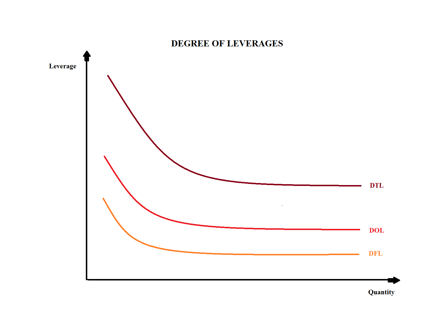
In the above equation, we can see that the degree of total leverage is significantly higher than the other two measures of leverages. This is mainly because the DTL is DOL multiplied by DFL.