a.  We can use the binomial model if we want to set up a portfolio of stock and an option in such a way that there is no uncertainty about the value at termination.

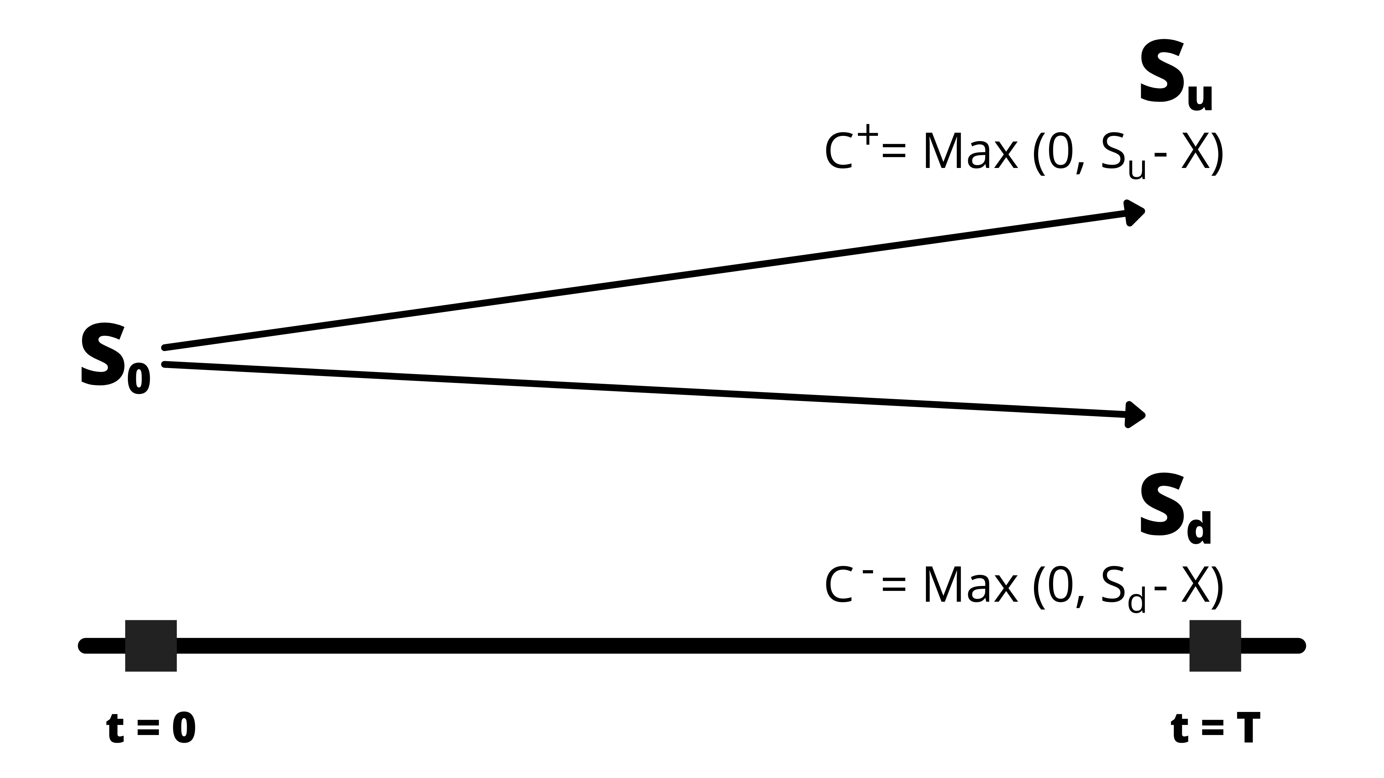
b.  Suppose we have an asset with a spot price of S_o, and it can be expected that the spot price may either go up to S_u, or may go down to S_d.

Also suppose the asset holder has also issued a corresponding option for the asset, which would have a maximum value of C⁺ = Max(0, S_u – X) at the termination date if the value goes up, and a maximum value of C^– = Max (0, S_d – X) at the termination date if the value goes down.

Suppose we begin with a portfolio nS number of the underlying asset and sell C number of options.

Suppose at the termination, if the value of the asset goes up, the value of the portfolio would be:

V_u = nS_u – C⁺

If, however, the value of the stock goes down, the value of the portfolio would be:

V_d = nS_d – C^–

As per the binomial model, whatever is the price of the underlying asset at the termination of the contract, the value of the portfolio should remain the same. Thus

nS_u – C⁺=  nS_d – C^–

We can now re-write this equation as:

nS_u – nS_d=  C⁺– C^–

Or,

n =  (C⁺– C^–) / (S_u – S_d)

The above equation represents the number of shares that should be bought so that at the termination the value of the portfolio is the same under both the circumstances, whether the price falls up or down.

We can also write the above equation as:

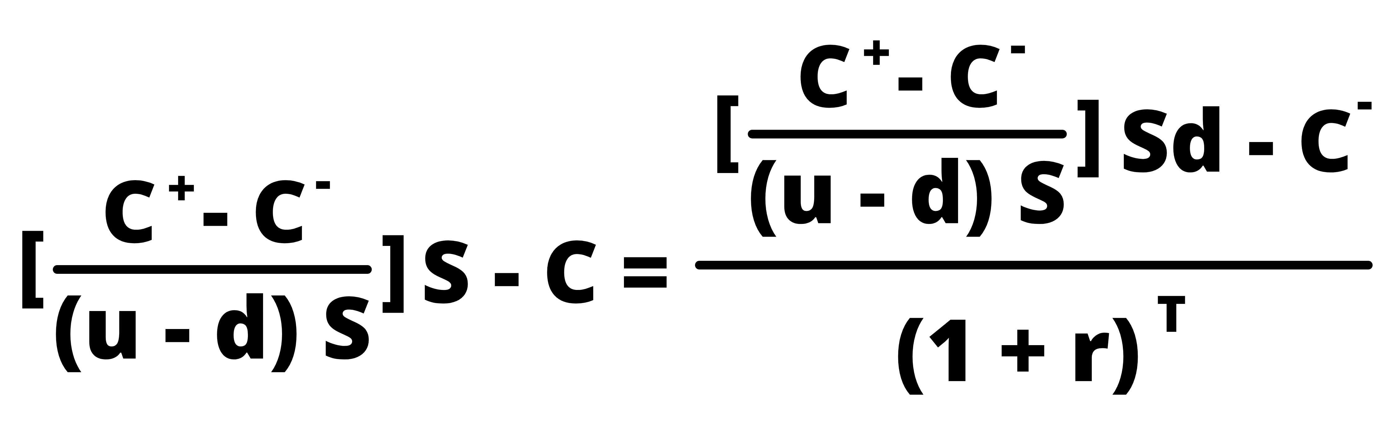
n =  (C⁺– C^–) / [(u-d) S] 

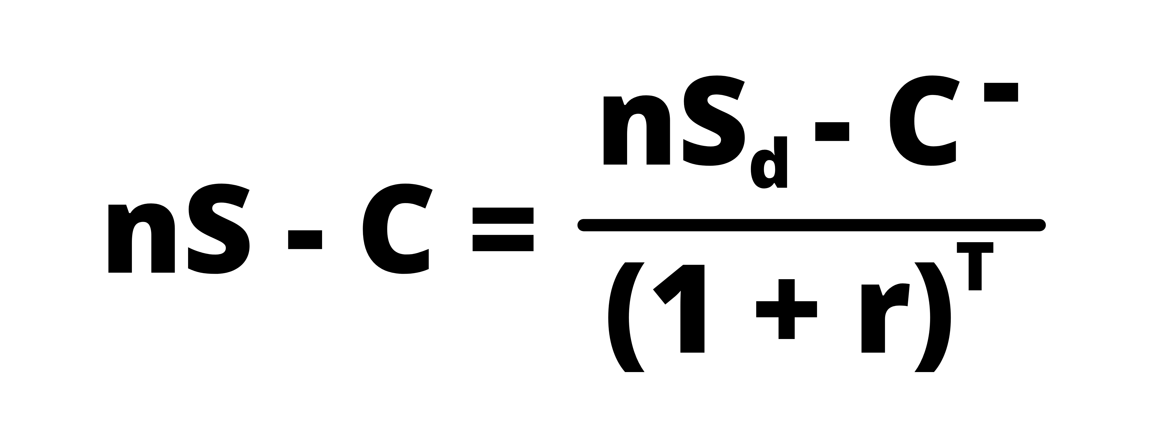
c.  At the time t = 0, the value of the portfolio is ‘nS-C’. Whereas, at the termination date, i.e. t = T, the value of the portfolio is ‘nSd – C^–’, if the price goes down. The present value of this equation should equal the current value of the portfolio, in the absence of arbitrage. Therefore,

If we now replace the value of ‘n’ in the above equation with the value of ‘n’ derived in the previous point, then:

We can simplify this equation to the following:

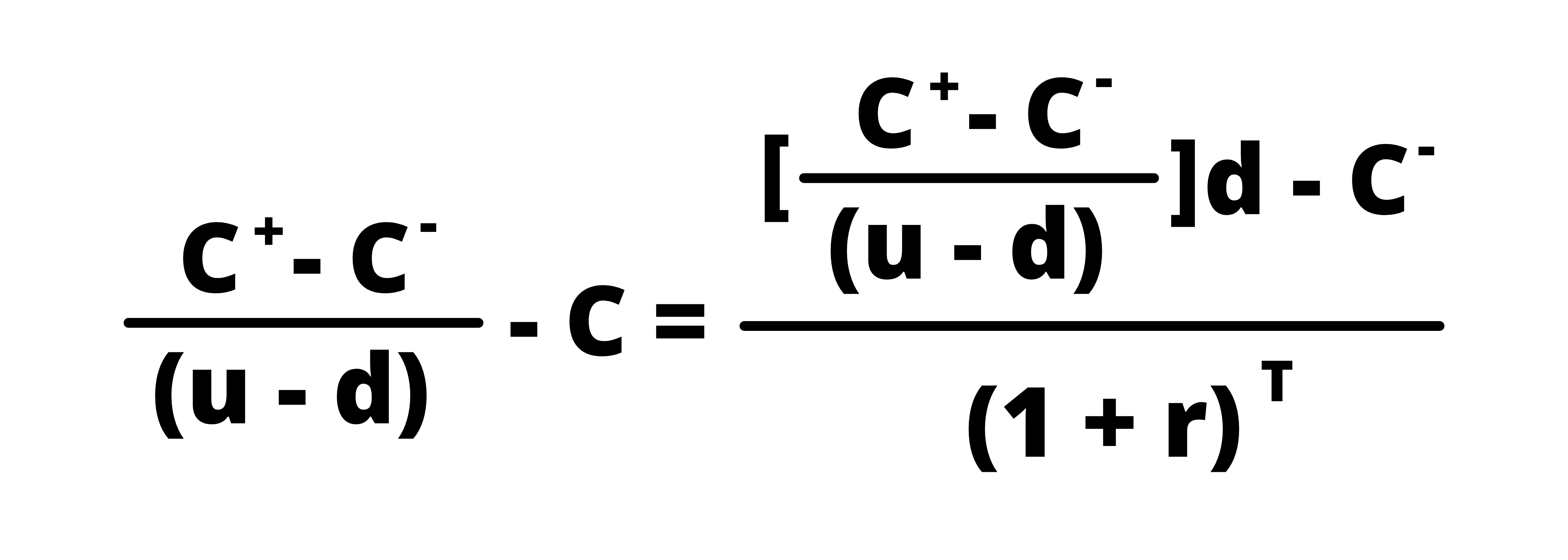
Here we are trying to find the value of C. Thus,

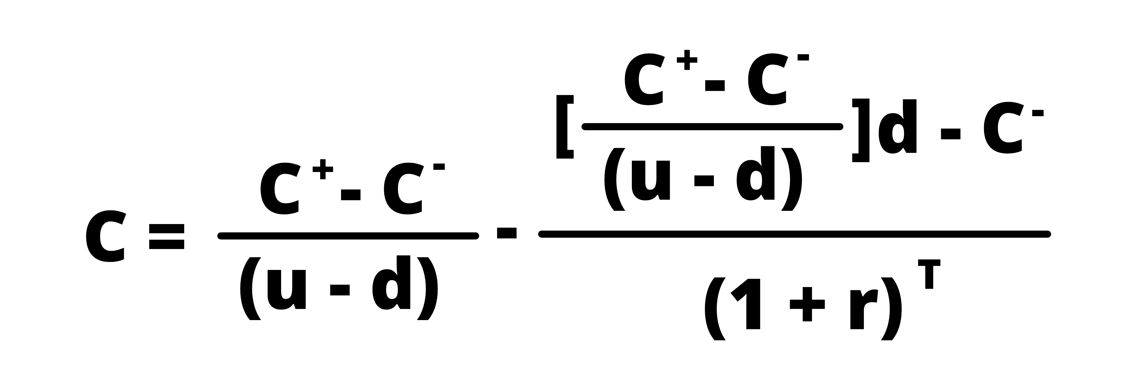
If we solve the following equation, we get:

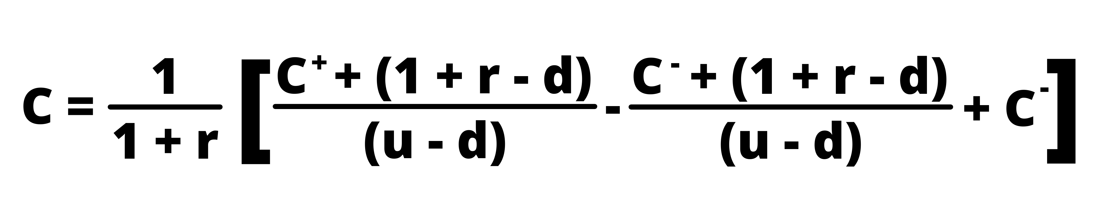
Let, ℼ = (1 + r – d) / (u – d)

So, we can write the above equation as:

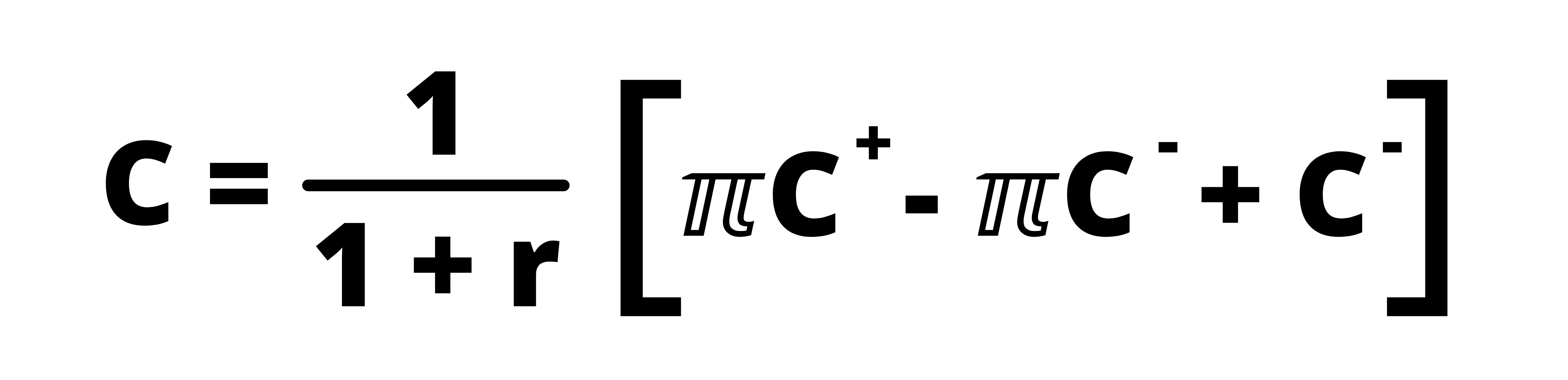
Or,

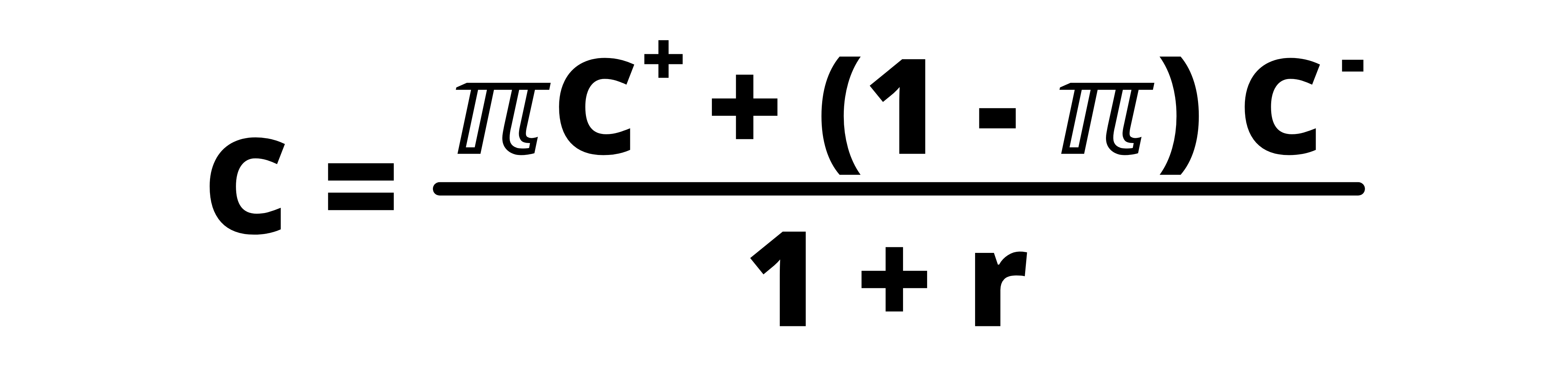
Here, ‘π’ and ‘1-π’ are nothing but the risk-neutral probabilities, and the term ‘u-d’ represents the volatility.

Example:

To explain the above, let us suppose that we have an asset that has a current spot price is $100. The risk-free rate prevailing in the market is 5%. We must find the at-the-money call price, assuming that the stock price may go either up or down by 20%.

So, we have the following information available:

Now, we can find the value of π using the above formula,

ℼ = (1 + r – d) / (u – d) = (1+0.05-0.80)/(1.20 – 0.80) = 0.625

Putting this value of π in the equation

= [(0.625*20) + (1-0.625)*0] / (1+0.05) 

We get the value of C = 11.90

d.  One period binomial arbitrage opportunity

     i.  If the price of the call option is greater than the model price (i.e. C₀ > model price) then the investors seeking the arbitrage opportunity would sell the call options and buy the ‘n’ number of underlying assets.

    ii.  If the price of the call option is less than the model price (i.e. C₀ < model price) then the investors seeking the arbitrage opportunity would buy the call options by selling the ‘n’ number of underlying assets.

e.  If we want to use the binomial model for put option pricing, we follow the same process, except, instead of using C⁺/ C^–, we use P⁺/P^–, which is Max (0, X-S_T).