Course Content
THE TIME VALUE OF MONEY
This chapter is covered in reading 6 of study session 2 of the material provided by the institute. After reading this chapter, a student should be able to: a) interpret interest rates as required rates of return, discount rates, or opportunity costs; b) explain an interest rate as the sum of a real risk-free rate and premiums that compensate investors for bearing distinct types of risk; c) calculate and interpret the effective annual rate, given the stated annual interest rate and the frequency of compounding; d) solve time value of money problems for different frequencies of compounding; e) calculate and interpret the future value (FV) and present value (PV) of a single sum of money, an ordinary annuity, an annuity due, perpetuity (PV only), and a series of unequal cash flows; f) demonstrate the use of a timeline in modeling and solving time value of money problems.
0/2
STATISTICAL CONCEPTS AND MARKET RETURNS
This chapter is covered in reading 7 of study session 2 of the material provided by the Institute. After reading this chapter, a student should be able to: a. distinguish between descriptive statistics and inferential statistics, between a population and a sample, and among the types of measurement scales; b. define a parameter, a sample statistic, and a frequency distribution; c. calculate and interpret relative frequencies and cumulative relative frequencies, given a frequency distribution; d. describe the properties of a data set presented as a histogram or a frequency polygon; e. calculate and interpret measures of central tendency, including the population mean, the sample mean, arithmetic mean, weighted average or mean, geometric mean, harmonic mean, median, and mode; f. calculate and interpret quartiles, quintiles, deciles, and percentiles; g. calculate and interpret 1) a range and a mean absolute deviation and 2) the variance and standard deviation of a population and of a sample; h. calculate and interpret the proportion of observations falling within a specified number of standard deviations of the mean using Chebyshev’s inequality; i. calculate and interpret the coefficient of variation and the Sharpe ratio; j. explain skewness and the meaning of a positively or negatively skewed return distribution; k. describe the relative locations of the mean, median, and mode for a unimodal, nonsymmetrical distribution; l. explain measures of sample skewness and kurtosis; m. compare the use of arithmetic and geometric means when analyzing investment returns.
0/9
PROBABILITY CONCEPTS
This chapter is covered in reading 8 of study session 2 of the material provided by the Institute. After reading this chapter, a student should be able to: a. define a random variable, an outcome, an event, mutually exclusive events, and exhaustive events; b. state the two defining properties of probability and distinguish among empirical, subjective, and a priori probabilities; c. state the probability of an event in terms of odds for and against the event; d. distinguish between unconditional and conditional probabilities; e. explain the multiplication, addition, and total probability rules; f. calculate and interpret 1) the joint probability of two events, 2) the probability that at least one of two events will occur, given the probability of each and the joint probability of the two events, and 3) a joint probability of any number of independent events; g. distinguish between dependent and independent events; h. calculate and interpret an unconditional probability using the total probability rule; i. explain the use of conditional expectation in investment applications; j. explain the use of a tree diagram to represent an investment problem; k. calculate and interpret covariance and correlation; l. calculate and interpret the expected value, variance, and standard deviation of a random variable and of returns on a portfolio; m. calculate and interpret covariance given a joint probability function; n. calculate and interpret an updated probability using Bayes’ formula; o. identify the most appropriate method to solve a particular counting problem and solve counting problems using factorial, combination, and permutation concepts.
0/9
COMMON PROBABILITY DISTRIBUTIONS
This chapter is covered under reading 9, study session 3, as provided by the institute. After reading this chapter, a student shall be able to: a. define a probability distribution and distinguish between discrete and continuous random variables and their probability functions; b. describe the set of possible outcomes of a specified discrete random variable; c. interpret a cumulative distribution function; d. calculate and interpret probabilities for a random variable, given its cumulative distribution function; e. define a discrete uniform random variable, a Bernoulli random variable, and a binomial random variable; f. calculate and interpret probabilities given the discrete uniform and the binomial distribution functions; g. construct a binomial tree to describe stock price movement; h. calculate and interpret tracking error; i. define the continuous uniform distribution and calculate and interpret probabilities, given a continuous uniform distribution; j. explain the key properties of the normal distribution; k. distinguish between a univariate and a multivariate distribution and explain the role of correlation in the multivariate normal distribution; l. determine the probability that a normally distributed random variable lies inside a given interval; m. define the standard normal distribution, explain how to standardize a random variable, and calculate and interpret probabilities using the standard normal distribution; n. define shortfall risk, calculate the safety-first ratio, and select an optimal portfolio using Roy’s safety-first criterion; o. explain the relationship between normal and lognormal distributions and why the lognormal distribution is used to model asset prices; p. distinguish between discretely and continuously compounded rates of return and calculate and interpret a continuously compounded rate of return, given a specific holding period return; q. explain Monte Carlo simulation and describe its applications and limitations; r. compare Monte Carlo simulation and historical simulation.
0/6
SAMPLING AND ESTIMATION
This chapter is covered under reading 10, study session 3, as provided by the institute. After reading this chapter, a student shall be able to: a. define simple random sampling and a sampling distribution; b. explain sampling error; c. distinguish between simple random and stratified random sampling; d. distinguish between time-series and cross-sectional data; e. explain the central limit theorem and its importance; f. calculate and interpret the standard error of the sample mean; g. identify and describe desirable properties of an estimator; h. distinguish between a point estimate and a confidence interval estimate of a population parameter; i. describe properties of Student’s t-distribution and calculate and interpret its degrees of freedom; j. calculate and interpret a confidence interval for a population mean, given a normal distribution with 1) a known population variance, 2) an unknown population variance, or 3) an unknown variance and a large sample size; k. describe the issues regarding selection of the appropriate sample size, data mining bias, sample selection bias, survivorship bias, look-ahead bias, and time-period bias.
0/7
HYPOTHESIS TESTING
This chapter is covered under reading 11, study session 3, as provided by the institute. After reading this chapter, a student shall be able to: a. define a hypothesis, describe the steps of hypothesis testing, and describe and interpret the choice of the null and alternative hypotheses; b. distinguish between one-tailed and two-tailed tests of hypotheses; c. explain a test statistic, Type I and Type II errors, a significance level, and how significance levels are used in hypothesis testing; d. explain a decision rule, the power of a test, and the relation between confidence intervals and hypothesis tests; e. distinguish between a statistical result and an economically meaningful result; f. explain and interpret the p-value as it relates to hypothesis testing; g. identify the appropriate test statistic and interpret the results for a hypothesis test concerning the population mean of both large and small samples when the population is normally or approximately normally distributed and the variance is 1) known or 2) unknown; h. identify the appropriate test statistic and interpret the results for a hypothesis test concerning the equality of the population means of two at least approximately normally distributed populations, based on independent random samples with 1) equal or 2) unequal assumed variances; i. identify the appropriate test statistic and interpret the results for a hypothesis test concerning the mean difference of two normally distributed populations; j. identify the appropriate test statistic and interpret the results for a hypothesis test concerning 1) the variance of a normally distributed population, and 2) the equality of the variances of two normally distributed populations based on two independent random samples; k. formulate a test of the hypothesis that the population correlation coefficient equals zero and determine whether the hypothesis is rejected at a given level of significance; l. distinguish between parametric and nonparametric tests and describe situations in which the use of nonparametric tests may be appropriate.
0/8
Quantitative Methods
About Lesson

LOS J requires us to:

identify the appropriate test statistic and interpret the results for a hypothesis test concerning 1) the variance of a normally distributed population, and 2) the equality of the variances of two normally distributed populations based on two independent random samples


There are two types of tests for variances, i.e. tests concerning the value of single population variance and tests concerning the differences between two population variances.

1.  Testing a Single Variance

a.  The hypothesis for testing the variance is:

i.hypothesis for testing the variance  Quantitative Methods CFA level 1 Study Notes  

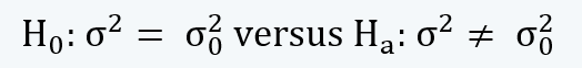
(a “not equal to” alternative hypothesis)

ii.  hypothesis for testing the variance  Quantitative Methods CFA level 1 Study Notes

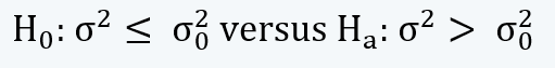
 (a “greater than” alternative hypothesis)

iii.  hypothesis for testing the variance  Quantitative Methods CFA level 1 Study Notes

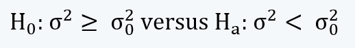
(a “less than” alternative hypothesis)

b.  The test for single variance is done using chi-square test statistics, which is denoted by χ2.

c.  As the value of the variance cannot be negative (since it has a square figure in the numerator and a positive number in the denominator), the value of the test statistic of chi-square is also greater than zero.

Thus we can say that the distribution of chi-square is bounded by zero in the left tail and has an extended right tail.

Chi-Square Test Quantitative Methods CFA level 1 Study Notes

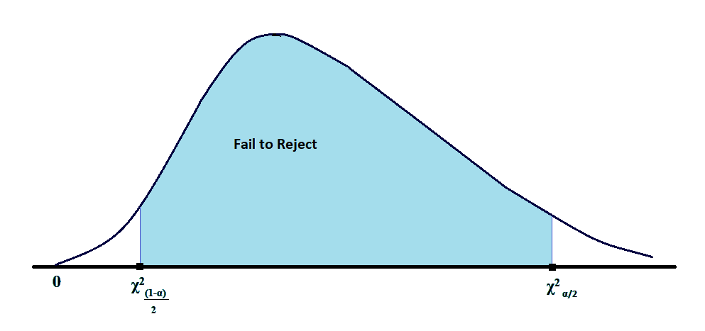
In the above figure, if the test was one-tailed, instead of two-tailed, it would have been α or (1-α) instead of α/2 or (1-α)/2

d.  The test statistic for the chi-square test is:

Chi-Square Test Quantitative Methods CFA level 1 Study Notes

e.  The chi-square test for single variance is done with a degree of freedom of n-1 and is very sensitive to the underlying assumptions.

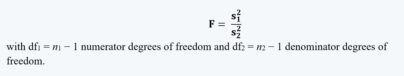
2.  Tests Comparing Two Variance Measures

a.  Tests for comparing two variances are conducted if we have two normally distributed populations with means μ1and μ2 and variances σ12 and σ22.

b.  The hypothesis for this test is written as follows:

Hypothesis Testing Quantitative Methods CFA level 1 Study Notes

c.  Note that, in the hypothesis, H0: σ12 = σ22, we have H0: σ12 / σ22 =1.

d.  Therefore the test statistic for the test of two variances (i.e. f-test statistic) is:

f-test statistic  Quantitative Methods CFA level 1 Study Notes
e.  Since the f-statistic is the ratio between the two variances, and this ratio does affect the curvature of the distribution. Now, the question is which sample’s variance should be chosen as the numerator for the calculations?

The answer is that we should choose the sample with a larger variance as the numerator.

f.   Finally, we make the decision as follows:

‘if the test statistic is greater than the critical value for an F-distribution with df1 and df2 degrees of freedom, reject the null hypothesis’.