LOS J requires us to:
j. explain skewness and the meaning of a positively or negatively skewed return distribution
k. describe the relative locations of the mean, median, and mode for a unimodal, nonsymmetrical distribution;
a. Skewness measures the degree of symmetry in return distribution.
b. Depending upon the skewness, a frequency distribution could be symmetrical or non-symmetrical.
c. A symmetrical distribution or normal distribution curve has the following characteristics:
i. It is bell-shaped.
ii. Its mean is equal to its median.
iii. A symmetrical distribution is completely described by the two parameters, i.e. mean and variance.
A graph of a typical normal distribution curve looks like this:
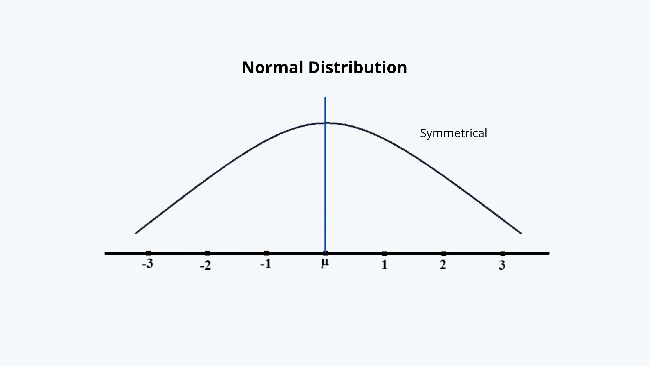
In such a distribution typically 68.3% of the observations lie between + and – 1, 95.5% between + and – 2, and 99.7% between + and -3.
d. A non-symmetrical could be of two types, i.e. positively skewed or negatively skewed.
A typical positively skewed distribution curve looks like this:
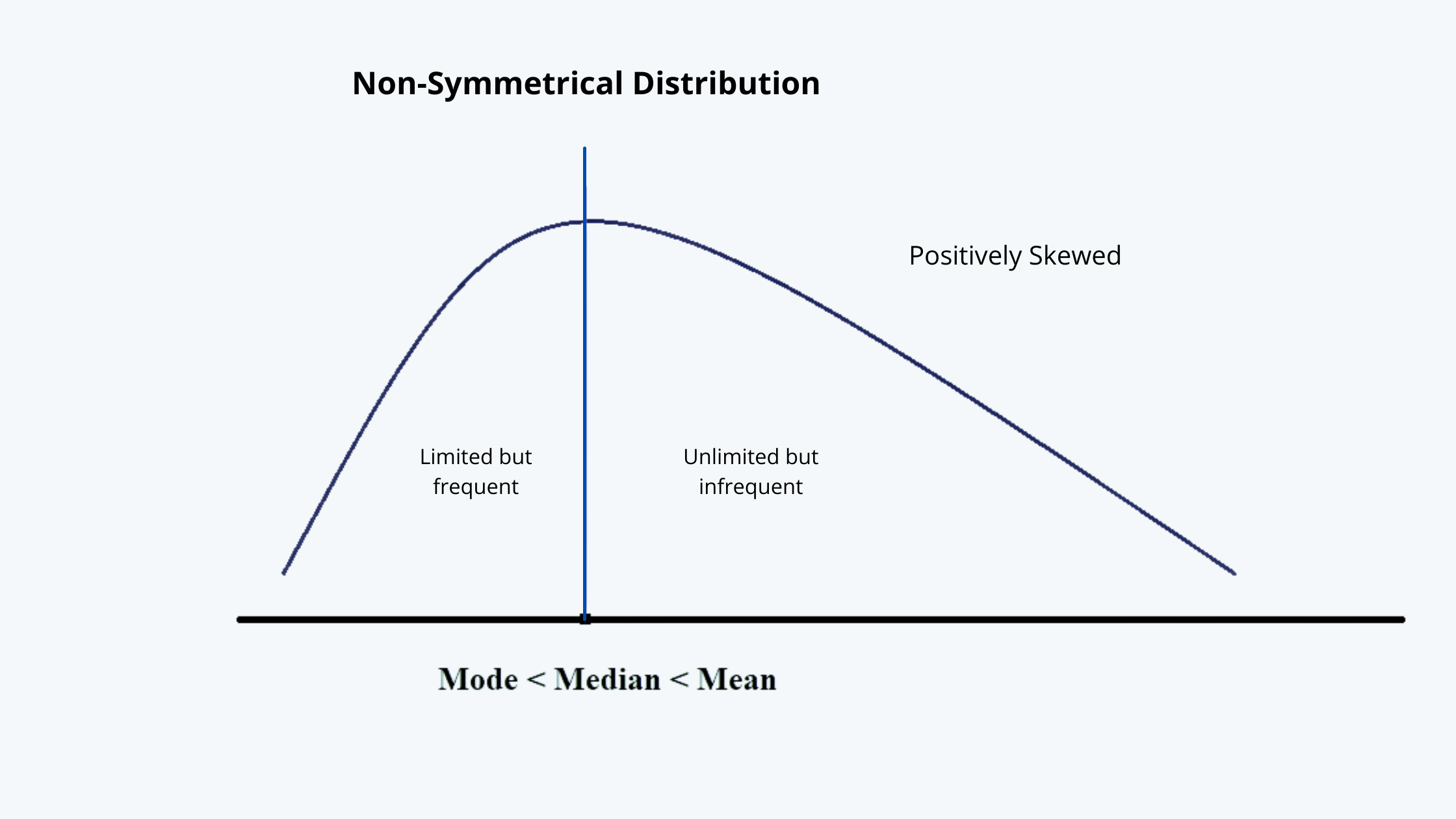
Such a distribution is characterized by:
i. Limited but frequent negative returns and unlimited but infrequent positive returns.
ii. In such a distribution the mode is less than the median and median less than the mean.
A positively skewed distribution pattern can be observed in buying a call and put options.
A typical negatively skewed distribution curve looks like this:
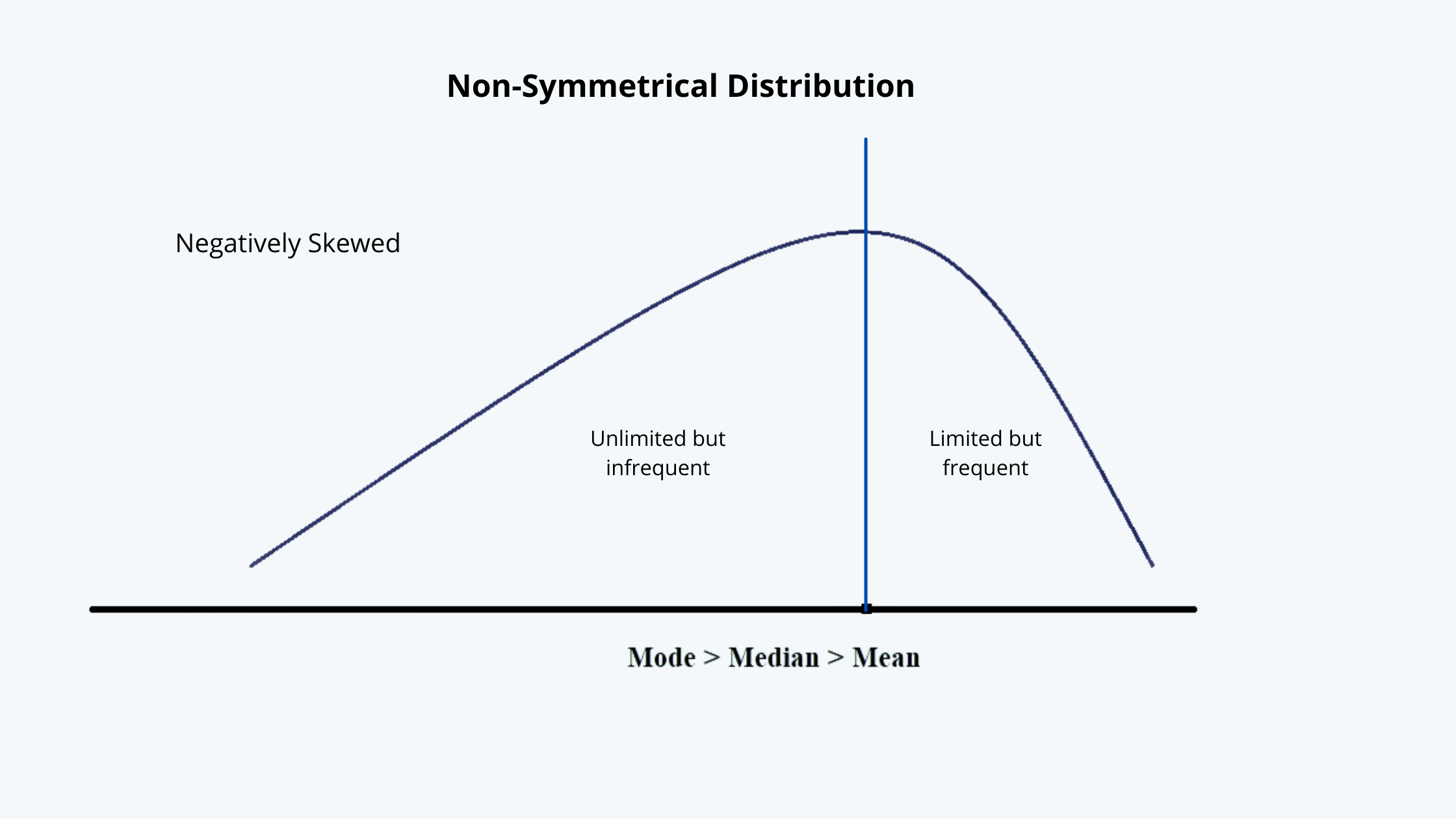
Such a distribution is characterized by:
i. Limited but frequent positive returns and unlimited but infrequent negative returns.
ii. In such a distribution the mode is more than the median and median more than the mean.
A positively skewed distribution pattern can be observed in selling call and put options.
e. The formula for calculating the skewness of a frequency distribution is:

In the above equation:
i. We take the cube root of the term (Xi – Ẍ) in order to preserve the sign (positive or negative) of the deviation; and thus, we take the cube root of s (i.e. sample standard deviation) as well.
ii. As the n gets larger, the value n / [(n-1) (n-2)] of gets closer to 1/(n-3) .
iii. If the skewness is 0, then it is a symmetrical distribution, and the average magnitude of positive deviation is equal to the average magnitude of the negative deviations.
iv. If the skewness is less than zero and the average magnitude of positive deviation is less than the average magnitude of the negative deviations, and it is a negatively skewed distribution.
v. If the skewness is more than zero and the average magnitude of negative deviation is less than the average magnitude of the positive deviations, and it is a positively skewed distribution.
vi. For distribution with n greater than 100, the skewness of ± 0.5 is considered as large.