Course Content
THE TIME VALUE OF MONEY
This chapter is covered in reading 6 of study session 2 of the material provided by the institute. After reading this chapter, a student should be able to: a) interpret interest rates as required rates of return, discount rates, or opportunity costs; b) explain an interest rate as the sum of a real risk-free rate and premiums that compensate investors for bearing distinct types of risk; c) calculate and interpret the effective annual rate, given the stated annual interest rate and the frequency of compounding; d) solve time value of money problems for different frequencies of compounding; e) calculate and interpret the future value (FV) and present value (PV) of a single sum of money, an ordinary annuity, an annuity due, perpetuity (PV only), and a series of unequal cash flows; f) demonstrate the use of a timeline in modeling and solving time value of money problems.
0/2
STATISTICAL CONCEPTS AND MARKET RETURNS
This chapter is covered in reading 7 of study session 2 of the material provided by the Institute. After reading this chapter, a student should be able to: a. distinguish between descriptive statistics and inferential statistics, between a population and a sample, and among the types of measurement scales; b. define a parameter, a sample statistic, and a frequency distribution; c. calculate and interpret relative frequencies and cumulative relative frequencies, given a frequency distribution; d. describe the properties of a data set presented as a histogram or a frequency polygon; e. calculate and interpret measures of central tendency, including the population mean, the sample mean, arithmetic mean, weighted average or mean, geometric mean, harmonic mean, median, and mode; f. calculate and interpret quartiles, quintiles, deciles, and percentiles; g. calculate and interpret 1) a range and a mean absolute deviation and 2) the variance and standard deviation of a population and of a sample; h. calculate and interpret the proportion of observations falling within a specified number of standard deviations of the mean using Chebyshev’s inequality; i. calculate and interpret the coefficient of variation and the Sharpe ratio; j. explain skewness and the meaning of a positively or negatively skewed return distribution; k. describe the relative locations of the mean, median, and mode for a unimodal, nonsymmetrical distribution; l. explain measures of sample skewness and kurtosis; m. compare the use of arithmetic and geometric means when analyzing investment returns.
0/9
PROBABILITY CONCEPTS
This chapter is covered in reading 8 of study session 2 of the material provided by the Institute. After reading this chapter, a student should be able to: a. define a random variable, an outcome, an event, mutually exclusive events, and exhaustive events; b. state the two defining properties of probability and distinguish among empirical, subjective, and a priori probabilities; c. state the probability of an event in terms of odds for and against the event; d. distinguish between unconditional and conditional probabilities; e. explain the multiplication, addition, and total probability rules; f. calculate and interpret 1) the joint probability of two events, 2) the probability that at least one of two events will occur, given the probability of each and the joint probability of the two events, and 3) a joint probability of any number of independent events; g. distinguish between dependent and independent events; h. calculate and interpret an unconditional probability using the total probability rule; i. explain the use of conditional expectation in investment applications; j. explain the use of a tree diagram to represent an investment problem; k. calculate and interpret covariance and correlation; l. calculate and interpret the expected value, variance, and standard deviation of a random variable and of returns on a portfolio; m. calculate and interpret covariance given a joint probability function; n. calculate and interpret an updated probability using Bayes’ formula; o. identify the most appropriate method to solve a particular counting problem and solve counting problems using factorial, combination, and permutation concepts.
0/9
COMMON PROBABILITY DISTRIBUTIONS
This chapter is covered under reading 9, study session 3, as provided by the institute. After reading this chapter, a student shall be able to: a. define a probability distribution and distinguish between discrete and continuous random variables and their probability functions; b. describe the set of possible outcomes of a specified discrete random variable; c. interpret a cumulative distribution function; d. calculate and interpret probabilities for a random variable, given its cumulative distribution function; e. define a discrete uniform random variable, a Bernoulli random variable, and a binomial random variable; f. calculate and interpret probabilities given the discrete uniform and the binomial distribution functions; g. construct a binomial tree to describe stock price movement; h. calculate and interpret tracking error; i. define the continuous uniform distribution and calculate and interpret probabilities, given a continuous uniform distribution; j. explain the key properties of the normal distribution; k. distinguish between a univariate and a multivariate distribution and explain the role of correlation in the multivariate normal distribution; l. determine the probability that a normally distributed random variable lies inside a given interval; m. define the standard normal distribution, explain how to standardize a random variable, and calculate and interpret probabilities using the standard normal distribution; n. define shortfall risk, calculate the safety-first ratio, and select an optimal portfolio using Roy’s safety-first criterion; o. explain the relationship between normal and lognormal distributions and why the lognormal distribution is used to model asset prices; p. distinguish between discretely and continuously compounded rates of return and calculate and interpret a continuously compounded rate of return, given a specific holding period return; q. explain Monte Carlo simulation and describe its applications and limitations; r. compare Monte Carlo simulation and historical simulation.
0/6
SAMPLING AND ESTIMATION
This chapter is covered under reading 10, study session 3, as provided by the institute. After reading this chapter, a student shall be able to: a. define simple random sampling and a sampling distribution; b. explain sampling error; c. distinguish between simple random and stratified random sampling; d. distinguish between time-series and cross-sectional data; e. explain the central limit theorem and its importance; f. calculate and interpret the standard error of the sample mean; g. identify and describe desirable properties of an estimator; h. distinguish between a point estimate and a confidence interval estimate of a population parameter; i. describe properties of Student’s t-distribution and calculate and interpret its degrees of freedom; j. calculate and interpret a confidence interval for a population mean, given a normal distribution with 1) a known population variance, 2) an unknown population variance, or 3) an unknown variance and a large sample size; k. describe the issues regarding selection of the appropriate sample size, data mining bias, sample selection bias, survivorship bias, look-ahead bias, and time-period bias.
0/7
HYPOTHESIS TESTING
This chapter is covered under reading 11, study session 3, as provided by the institute. After reading this chapter, a student shall be able to: a. define a hypothesis, describe the steps of hypothesis testing, and describe and interpret the choice of the null and alternative hypotheses; b. distinguish between one-tailed and two-tailed tests of hypotheses; c. explain a test statistic, Type I and Type II errors, a significance level, and how significance levels are used in hypothesis testing; d. explain a decision rule, the power of a test, and the relation between confidence intervals and hypothesis tests; e. distinguish between a statistical result and an economically meaningful result; f. explain and interpret the p-value as it relates to hypothesis testing; g. identify the appropriate test statistic and interpret the results for a hypothesis test concerning the population mean of both large and small samples when the population is normally or approximately normally distributed and the variance is 1) known or 2) unknown; h. identify the appropriate test statistic and interpret the results for a hypothesis test concerning the equality of the population means of two at least approximately normally distributed populations, based on independent random samples with 1) equal or 2) unequal assumed variances; i. identify the appropriate test statistic and interpret the results for a hypothesis test concerning the mean difference of two normally distributed populations; j. identify the appropriate test statistic and interpret the results for a hypothesis test concerning 1) the variance of a normally distributed population, and 2) the equality of the variances of two normally distributed populations based on two independent random samples; k. formulate a test of the hypothesis that the population correlation coefficient equals zero and determine whether the hypothesis is rejected at a given level of significance; l. distinguish between parametric and nonparametric tests and describe situations in which the use of nonparametric tests may be appropriate.
0/8
Quantitative Methods
About Lesson

LOS A, B, and C requires us to:

a.  define simple random sampling and a sampling distribution
b.  explain sampling error
c.  distinguish between simple random and stratified random sampling


Before, we understand the methodology and technique of sampling; it is important to understand its concepts. These concepts include parameters, statistics, and samples.

1.  Parameters & Statistics

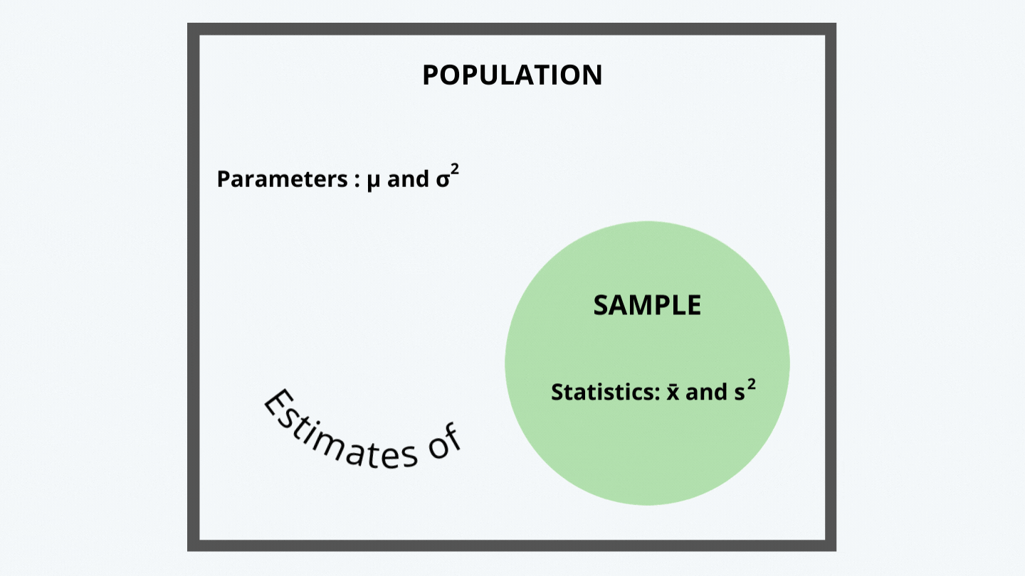
a.  All the data concerning information is called the population of the data.

b.  The parameters are the measurable characteristics of the entire population data, such as its mean and variance.

The population mean and variance is generally denoted by the sign µ and σ2.

c.  A parameter is a quantity used to describe a population, and a statistic is a quantity computed from a sample and is used to estimate a population parameter and describe the sample.

d.  The sample statistics are used to estimate the parameters because it is not always feasible and possible to examine the entire population. It could be just too expensive to do the same.

We, thus, calculate the sample mean and sample variance, generally denoted by the symbols x̄ and s2.

e.  Consider the following figure:

Sample and population Quantitative Methods CFA level 1 Study Notes


f.  In order for a calculated statistic to convey information about the related population parameter, the sample should be chosen wisely to reflect the parameter’s characteristics. There are certain conditions that must be met; those conditions are generally satisfied if the sample used to calculate the statistics is random.

2.  Random Samples

a.  A simple random sample is a subset of the population drawn in such a way that each element of the population has an equal probability of being chosen.

b.  The simple random samples can be chosen using one of many techniques, such as:

i.  Using a random number generator, which generates certain numbers and those variables that lie on that number in the sequence get selected as a sample.

ii.   Using systematic sampling techniques, such as selecting every kth element in the sequence of variables.

c.  There are many different samples possible in the population and each of such sample’s mean and variance may not equal the other.

Distribution of Sample Mean Quantitative Methods CFA level 1 Study Notes

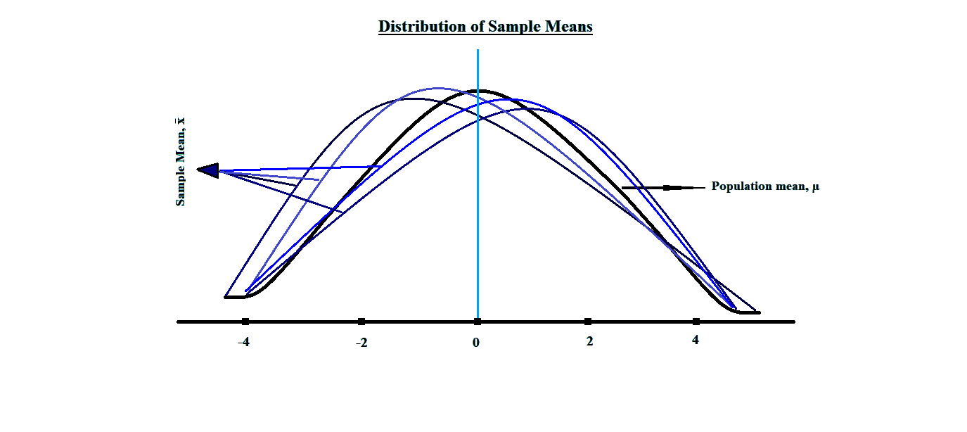
So that if we take a sample at random can calculate its mean and variance as and may not equal the other x̄2 and s22. Such that,

Distribution of Sample Mean Quantitative Methods CFA level 1 Study Notes

And, usually, none of the sample’s mean equals the population’s mean and variance. The means of all the samples in a data are usually distributed normally; and if we want to calculate the mean of the population using these sample’s mean, we would calculate the mean of the sample means, which is equal to the population mean. That is,

Distribution of Sample Mean Quantitative Methods CFA level 1 Study Notes

d.  Since the population mean is mostly not equal to the sample’s mean; therefore, there is always a difference between these two means. This difference between the population mean and the sample mean is called the sampling error. That is:

Sampling Error Quantitative Methods CFA level 1 Study Notes

e.  The difference between the observed value of a statistic and the value of the parameter is known as the sampling error.

3.  Stratified Random Sampling

a.  In a large population, we may have subpopulations, known as strata, for each of which the analysts want to ensure inclusion in a representative way in the sample.
To do so, we can use stratified sampling, wherein we draw simple random samples from each strata and then combine those samples to form the overall sample on which we perform our analysis.

Stratified Sampling Quantitative Methods CFA level 1 Study Notes

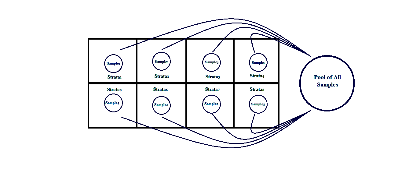
b.  The main steps involved in stratified random sampling are:

i.  Step 1: The population is first divided into sub-populations called the strata.

ii.  Step 2: Simple random samples are drawn from each strata in proportion to their size.

c.  Each of the strata, so divided, should be:

i.  Mutually exclusive, and

ii.  Collectively exhaustive.

d.  By using this technique, we get a sample that looks more like the population with more precise estimates of the sample mean and the variances (i.e. x̄ and s2). This is mainly because; the representativeness reduces the sampling error.