LOS L requires us to:

calculate and interpret the expected value, variance, and standard deviation of a random variable and of returns on a portfolio.

a.  Consider the following portfolio:

b.  The expected return on the portfolio is the weighted average of expected returns on different securities.

 Thus, for the above portfolio, the expected return would be:

c.  There is more than one asset or asset class in a portfolio. Some of the assets or asset classes may have a positively sloping yield curve, others may have a negatively sloping one. When more than one of such assets is combined, they may have a flat yield. This is mainly due to the covariance between the two. Thus, for calculating the portfolio variance one needs to calculate the covariance amongst different assets in the portfolio.

d.  Therefore, if we recall, the variance of a random variable is the probability-weighted average of squared deviation. Or,

A portfolio, however, is a collection of such random variables. For calculating the variance of such individual components, the above formula may be used. But, in order to calculate the variance of the portfolio, containing these individual variables, we need to calculate the covariance between each of such constituent variable.

e.  The covariance between the two assets in a portfolio is the probability-weighted average of the cross products. It can be calculated using the following formula:

f.  Using the covariance of each of the assets in the portfolio, the portfolio variance can also be calculated. The formula for calculating the portfolio variance is:

g.  If we have a three-asset portfolio, we would have a covariance matrix as follows:

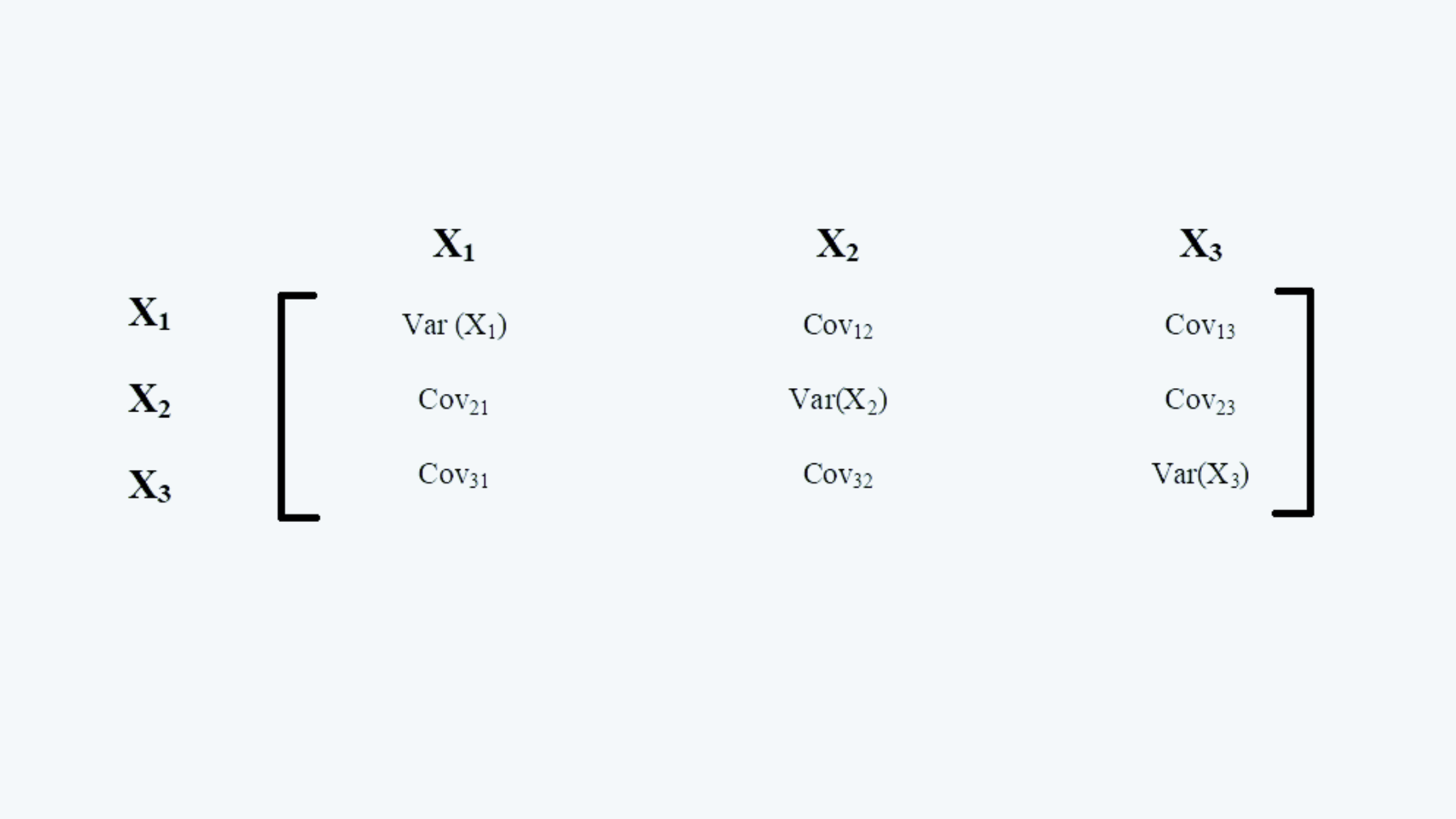
In the above covariance matrix, the following needs to be noted:

i.  The diagonal covariance, i.e. the covariance of the asset with itself is nothing but its variance.

ii.  The value of covariance between asset 1 & asset 2, and asset 2 & asset 1 (i.e. Cov_i,j & Cov_j,i) are the same.
Thus for a 3-asset matrix, we have 3 variances and three covariances to be calculated.
For a n-asset matrix, there would be n variances and

iii.  If the covariance between two assets is less than zero, they have an inverse relationship amongst them. If, however, there is a covariance greater than zero, they have a positive relationship.
If the covariance is zero, then there is no correlation between the assets.

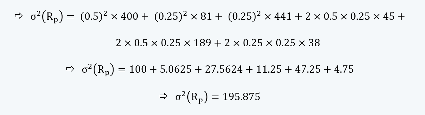
h.  Thus, if the above-mentioned portfolio has the following covariance matrix:

We can calculate the variance of the portfolio as follows:

i.  We can also calculate the correlation between the two assets using the following formula:

If we have to calculate the correlation matrix using the above covariance matrix, we can do so using the above formula. Thus the covariance between the asset 1 and 2 would be:

Similarly, the correlation between assets with themselves would always be 1. We can calculate the same as follows:

We can thus construct the correlation matrix on similar lines, as follows:

j.  Following need to be noted about the correlation between the two assets:

i.  The correlation between the two assets always ranges between +1 and -1.

ii.  A correlation of -1 indicates the perfect negative linear relationship between the two assets.

iii.  A correlation of +1 indicates the perfect positive linear relationship between the two assets.

iv.  A correlation of 0 indicates that there is no correlation between the two variables, whatsoever.