Course Content
THE TIME VALUE OF MONEY
This chapter is covered in reading 6 of study session 2 of the material provided by the institute. After reading this chapter, a student should be able to: a) interpret interest rates as required rates of return, discount rates, or opportunity costs; b) explain an interest rate as the sum of a real risk-free rate and premiums that compensate investors for bearing distinct types of risk; c) calculate and interpret the effective annual rate, given the stated annual interest rate and the frequency of compounding; d) solve time value of money problems for different frequencies of compounding; e) calculate and interpret the future value (FV) and present value (PV) of a single sum of money, an ordinary annuity, an annuity due, perpetuity (PV only), and a series of unequal cash flows; f) demonstrate the use of a timeline in modeling and solving time value of money problems.
0/2
STATISTICAL CONCEPTS AND MARKET RETURNS
This chapter is covered in reading 7 of study session 2 of the material provided by the Institute. After reading this chapter, a student should be able to: a. distinguish between descriptive statistics and inferential statistics, between a population and a sample, and among the types of measurement scales; b. define a parameter, a sample statistic, and a frequency distribution; c. calculate and interpret relative frequencies and cumulative relative frequencies, given a frequency distribution; d. describe the properties of a data set presented as a histogram or a frequency polygon; e. calculate and interpret measures of central tendency, including the population mean, the sample mean, arithmetic mean, weighted average or mean, geometric mean, harmonic mean, median, and mode; f. calculate and interpret quartiles, quintiles, deciles, and percentiles; g. calculate and interpret 1) a range and a mean absolute deviation and 2) the variance and standard deviation of a population and of a sample; h. calculate and interpret the proportion of observations falling within a specified number of standard deviations of the mean using Chebyshev’s inequality; i. calculate and interpret the coefficient of variation and the Sharpe ratio; j. explain skewness and the meaning of a positively or negatively skewed return distribution; k. describe the relative locations of the mean, median, and mode for a unimodal, nonsymmetrical distribution; l. explain measures of sample skewness and kurtosis; m. compare the use of arithmetic and geometric means when analyzing investment returns.
0/9
PROBABILITY CONCEPTS
This chapter is covered in reading 8 of study session 2 of the material provided by the Institute. After reading this chapter, a student should be able to: a. define a random variable, an outcome, an event, mutually exclusive events, and exhaustive events; b. state the two defining properties of probability and distinguish among empirical, subjective, and a priori probabilities; c. state the probability of an event in terms of odds for and against the event; d. distinguish between unconditional and conditional probabilities; e. explain the multiplication, addition, and total probability rules; f. calculate and interpret 1) the joint probability of two events, 2) the probability that at least one of two events will occur, given the probability of each and the joint probability of the two events, and 3) a joint probability of any number of independent events; g. distinguish between dependent and independent events; h. calculate and interpret an unconditional probability using the total probability rule; i. explain the use of conditional expectation in investment applications; j. explain the use of a tree diagram to represent an investment problem; k. calculate and interpret covariance and correlation; l. calculate and interpret the expected value, variance, and standard deviation of a random variable and of returns on a portfolio; m. calculate and interpret covariance given a joint probability function; n. calculate and interpret an updated probability using Bayes’ formula; o. identify the most appropriate method to solve a particular counting problem and solve counting problems using factorial, combination, and permutation concepts.
0/9
COMMON PROBABILITY DISTRIBUTIONS
This chapter is covered under reading 9, study session 3, as provided by the institute. After reading this chapter, a student shall be able to: a. define a probability distribution and distinguish between discrete and continuous random variables and their probability functions; b. describe the set of possible outcomes of a specified discrete random variable; c. interpret a cumulative distribution function; d. calculate and interpret probabilities for a random variable, given its cumulative distribution function; e. define a discrete uniform random variable, a Bernoulli random variable, and a binomial random variable; f. calculate and interpret probabilities given the discrete uniform and the binomial distribution functions; g. construct a binomial tree to describe stock price movement; h. calculate and interpret tracking error; i. define the continuous uniform distribution and calculate and interpret probabilities, given a continuous uniform distribution; j. explain the key properties of the normal distribution; k. distinguish between a univariate and a multivariate distribution and explain the role of correlation in the multivariate normal distribution; l. determine the probability that a normally distributed random variable lies inside a given interval; m. define the standard normal distribution, explain how to standardize a random variable, and calculate and interpret probabilities using the standard normal distribution; n. define shortfall risk, calculate the safety-first ratio, and select an optimal portfolio using Roy’s safety-first criterion; o. explain the relationship between normal and lognormal distributions and why the lognormal distribution is used to model asset prices; p. distinguish between discretely and continuously compounded rates of return and calculate and interpret a continuously compounded rate of return, given a specific holding period return; q. explain Monte Carlo simulation and describe its applications and limitations; r. compare Monte Carlo simulation and historical simulation.
0/6
SAMPLING AND ESTIMATION
This chapter is covered under reading 10, study session 3, as provided by the institute. After reading this chapter, a student shall be able to: a. define simple random sampling and a sampling distribution; b. explain sampling error; c. distinguish between simple random and stratified random sampling; d. distinguish between time-series and cross-sectional data; e. explain the central limit theorem and its importance; f. calculate and interpret the standard error of the sample mean; g. identify and describe desirable properties of an estimator; h. distinguish between a point estimate and a confidence interval estimate of a population parameter; i. describe properties of Student’s t-distribution and calculate and interpret its degrees of freedom; j. calculate and interpret a confidence interval for a population mean, given a normal distribution with 1) a known population variance, 2) an unknown population variance, or 3) an unknown variance and a large sample size; k. describe the issues regarding selection of the appropriate sample size, data mining bias, sample selection bias, survivorship bias, look-ahead bias, and time-period bias.
0/7
HYPOTHESIS TESTING
This chapter is covered under reading 11, study session 3, as provided by the institute. After reading this chapter, a student shall be able to: a. define a hypothesis, describe the steps of hypothesis testing, and describe and interpret the choice of the null and alternative hypotheses; b. distinguish between one-tailed and two-tailed tests of hypotheses; c. explain a test statistic, Type I and Type II errors, a significance level, and how significance levels are used in hypothesis testing; d. explain a decision rule, the power of a test, and the relation between confidence intervals and hypothesis tests; e. distinguish between a statistical result and an economically meaningful result; f. explain and interpret the p-value as it relates to hypothesis testing; g. identify the appropriate test statistic and interpret the results for a hypothesis test concerning the population mean of both large and small samples when the population is normally or approximately normally distributed and the variance is 1) known or 2) unknown; h. identify the appropriate test statistic and interpret the results for a hypothesis test concerning the equality of the population means of two at least approximately normally distributed populations, based on independent random samples with 1) equal or 2) unequal assumed variances; i. identify the appropriate test statistic and interpret the results for a hypothesis test concerning the mean difference of two normally distributed populations; j. identify the appropriate test statistic and interpret the results for a hypothesis test concerning 1) the variance of a normally distributed population, and 2) the equality of the variances of two normally distributed populations based on two independent random samples; k. formulate a test of the hypothesis that the population correlation coefficient equals zero and determine whether the hypothesis is rejected at a given level of significance; l. distinguish between parametric and nonparametric tests and describe situations in which the use of nonparametric tests may be appropriate.
0/8
Quantitative Methods
About Lesson

LOS E and F require us to:

e.  calculate and interpret measures of central tendency, including the population mean, the sample mean, arithmetic mean, weighted average or mean, geometric mean, harmonic mean, median, and mode.
f.  calculate and interpret quartiles, quintiles, deciles, and percentiles.


The measures of central tendencies are quantitative measures of location that specifies where the data is centered. Different measures of central tendencies are discussed below:

1.  Arithmetic Mean

a.  Arithmetic mean is the average of the data of numerical values. It is calculated using the following formula:

Arithmetic Mean Quantitative Methods CFA level 1 Study Notes

That is, the mean is the sum of all observations in data, divided by the number of observations.

b.  The arithmetic mean could either be calculated for the entire population or the sample of the population.

c.  The population mean can only be calculated if the population can be defined. It can be calculated by summing up all the data in the population and dividing it by the number of observations. Thus, a population mean can be calculated as follows:

Population Mean Quantitative Methods CFA level 1 Study Notes
The ‘µ’ here represents the parameter because it is the mean of all the data in the population and there is the least scope for the error.

d.  The other mean that can be calculated is the sample mean. The sample is a smaller data, selected from within the population that is a reflection of the population behavior. The sample mean can be calculated as follows:

Sample Mean Quantitative Methods CFA level 1 Study Notes

2.  Median

a.  Median is the value in the middle of the population or the sample.

b.  Median can be calculated by first arranging the observations in ascending order, and then finding the middle value of the series of observations.

c.  If the series has an odd number of observations, then the median is the observation that occupies the [(n + 1) / 2]th position.

d.  If, however, the series has an even number of observations, the median is the average of observations occupying the [(n / 2]th and [(n + 2) / 2]th position

3.  Mode

a.  The mode is the most frequently occurring observation in the population or the sample.

b.  The data could either have a single mode, i.e. it might be unimodal, or it might have multiple modes (such as bi-modal data).

c.  The mode is the only measure of central tendency that can be used with nominal or categorical data.

4.  Weighted Mean

The weighted mean is similar to the arithmetic mean, except that instead of each data point contributing equally to the average, the more influential data is given the higher weights.

Thus, if say a portfolio consists of two types of investments, i.e. equity and bonds. The stocks form 60% of the portfolio and bonds form 40%. If equities provide a return of 10% and bonds a return of 8%, then the arithmetic mean of the two would be:

(10 + 8) / 2 = 9%

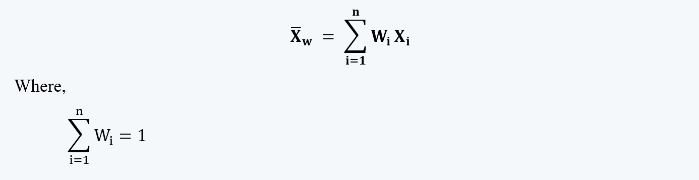
This average does not reflect the true weight of the individual components in the portfolio; therefore, it would be more appropriate to have a mean that gives weights to the individual categories in the portfolio. Thus, we calculate the weighted average instead of the arithmetic mean as follows:

Mean Example Quantitative Methods CFA level 1 Study Notes

Thus, the formula for calculating the weighted average is:

Weighted Average Formula Quantitative Methods CFA level 1 Study Notes

Example:

Consider a portfolio with 60% investment in equities and 40% in bonds. The different returns on equities and bonds for a period of 5 years were:

Year

Return on Equity

Return on Bonds

1

-2%

9%

2

8%

10%

3

27%

-1.5%

4

-9%

8%

5

-5%

7.5%

If we want to calculate the average returns earned by the investor, we should calculate the weighted average of the returns of each year and then take the arithmetic mean of the 5-year return.

Year

Return on Equity

Return on Bonds

Weighted Average (WiXi)

1

-2%

9%

2.4%

2

8%

10%

8.8%

3

27%

-1.5%

15.6%

4

-9%

8%

-2.2%

5

-5%

7.5%

0%

And the average of five year’s returns would be:

Weighted Average Example Quantitative Methods CFA level 1 Study Notes

5.  Geometric Mean

a.  It is the central number in a geometric progression. It is mostly used to average the ‘rates of change’, i.e. the growth rate of the variable.

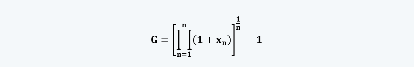
b.  The geometric mean is calculated by taking the nth root of the product of n numbers.

Geometric Mean formula Quantitative Methods CFA level 1 Study Notes

The geometric mean can be calculated as long as all the numbers in the data are greater than or equal to zero.

c.  In the above example, if we were to calculate the geometric mean of the equity investments we can calculate as follows:

Year

Return on Equity

1

-0.02

2

0.08

3

0.27

4

-0.09

5

-0.05

Since the returns are negative in some of the years; we should add 1 and then calculate the geometric mean. Thus,

Geometric Mean Example Quantitative Methods CFA level 1 Study Notes

Or, the average return on equity stocks was 3.05%.

d.  A general formula for calculation of geometric mean is:

Geometric Mean formula Quantitative Methods CFA level 1 Study Notes

or,

Geometric Mean General formula Quantitative Methods CFA level 1 Study Notes

6.  Comparison of Arithmetic and Geometric Mean

Suppose we begin our portfolio with a value of $ 100, at the end of year 1, it is worth $ 200 (i.e. 100% returns), and at the end of year 2, it is again worth $ 100 (i.e. a loss of 50% in the year 2).

So, if we calculate the arithmetic mean, the average returns would be:

Quantitative Methods CFA level 1 Study Notes STATISTICAL CONCEPTS AND MARKET RETURNS

And, if we calculate the geometric mean the average returns would be:

Quantitative Methods CFA level 1 Study Notes STATISTICAL CONCEPTS AND MARKET RETURNS

7.  Harmonic Mean

a.  Harmonic mean is another measure of central tendencies, but with very limited applications. They are mainly used for averaging the ratios, that too, only when they are repeatedly applied to a fixed quantity to yield a variable number of units.

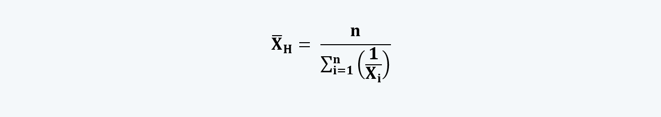
b.  The harmonic mean is usually calculated by taking the reciprocal of the reciprocals of the numbers in the set. The formula for calculating the harmonic mean is:

Harmonic Mean Quantitative Methods CFA level 1 Study Notes

c.  For example, if an investor has $ 1000 to invest every month and the price of a unit of the fund at the end of the first and second month is $ 10 and $ 15 respectively, so that he can buy 100 and 66.67 shares at the end of each month. To calculate the average price of the unit, the arithmetic mean is not appropriate here. Rather, we should calculate the harmonic mean of the price as follows:

Harmonic Mean Example Quantitative Methods CFA level 1 Study Notes

Thus, the average price of the fund is $ 12.

d.  While using the harmonic mean it is extremely important to understand the situations where the harmonic mean is used.

8.  Quantiles

a.  Quantiles refer to the set of variables that divide a frequency distribution into equal groups, having the same fraction of the total population.

b.  There are different types of quantiles; some of them are:

i.  Median: It divides the frequency distribution into two equal parts. It is the mid-point of the frequency distribution.

ii.  Quartile: The quartiles divide the frequency distribution into four equal parts.

iii.  Quintiles: They divide the frequency distribution into five equal parts.

iv.  Deciles: They divide the frequency distribution into ten equal parts.

v.  Percentiles: They divide the frequency distributions into the 100 equal parts

c.  Thus, for example when we say that a student in a class has obtained 70 percentile; it means that 70% of the students in the class have marks less than this student.

d.  Locating Percentiles:

The percentile points can be located using the following equation:

Locating Percentile Quantitative Methods CFA level 1 Study Notes

where y is the percentage point at which we are dividing the distribution and Ly is the location (L) of the percentile (Py) in the array sorted in ascending order.

e.  The point Ly may not be the whole number, and in such a case, we can locate the points using linear interpolation.

For example, if we know that observation 12 has the value of 20 and observation 13 has the value of 30. And if we have to find the value of observation 12.5, we can do so by interpolating the data as follows:

Locating Percentile Example Quantitative Methods CFA level 1 Study Notes