Course Content
THE TIME VALUE OF MONEY
This chapter is covered in reading 6 of study session 2 of the material provided by the institute. After reading this chapter, a student should be able to: a) interpret interest rates as required rates of return, discount rates, or opportunity costs; b) explain an interest rate as the sum of a real risk-free rate and premiums that compensate investors for bearing distinct types of risk; c) calculate and interpret the effective annual rate, given the stated annual interest rate and the frequency of compounding; d) solve time value of money problems for different frequencies of compounding; e) calculate and interpret the future value (FV) and present value (PV) of a single sum of money, an ordinary annuity, an annuity due, perpetuity (PV only), and a series of unequal cash flows; f) demonstrate the use of a timeline in modeling and solving time value of money problems.
0/2
STATISTICAL CONCEPTS AND MARKET RETURNS
This chapter is covered in reading 7 of study session 2 of the material provided by the Institute. After reading this chapter, a student should be able to: a. distinguish between descriptive statistics and inferential statistics, between a population and a sample, and among the types of measurement scales; b. define a parameter, a sample statistic, and a frequency distribution; c. calculate and interpret relative frequencies and cumulative relative frequencies, given a frequency distribution; d. describe the properties of a data set presented as a histogram or a frequency polygon; e. calculate and interpret measures of central tendency, including the population mean, the sample mean, arithmetic mean, weighted average or mean, geometric mean, harmonic mean, median, and mode; f. calculate and interpret quartiles, quintiles, deciles, and percentiles; g. calculate and interpret 1) a range and a mean absolute deviation and 2) the variance and standard deviation of a population and of a sample; h. calculate and interpret the proportion of observations falling within a specified number of standard deviations of the mean using Chebyshev’s inequality; i. calculate and interpret the coefficient of variation and the Sharpe ratio; j. explain skewness and the meaning of a positively or negatively skewed return distribution; k. describe the relative locations of the mean, median, and mode for a unimodal, nonsymmetrical distribution; l. explain measures of sample skewness and kurtosis; m. compare the use of arithmetic and geometric means when analyzing investment returns.
0/9
PROBABILITY CONCEPTS
This chapter is covered in reading 8 of study session 2 of the material provided by the Institute. After reading this chapter, a student should be able to: a. define a random variable, an outcome, an event, mutually exclusive events, and exhaustive events; b. state the two defining properties of probability and distinguish among empirical, subjective, and a priori probabilities; c. state the probability of an event in terms of odds for and against the event; d. distinguish between unconditional and conditional probabilities; e. explain the multiplication, addition, and total probability rules; f. calculate and interpret 1) the joint probability of two events, 2) the probability that at least one of two events will occur, given the probability of each and the joint probability of the two events, and 3) a joint probability of any number of independent events; g. distinguish between dependent and independent events; h. calculate and interpret an unconditional probability using the total probability rule; i. explain the use of conditional expectation in investment applications; j. explain the use of a tree diagram to represent an investment problem; k. calculate and interpret covariance and correlation; l. calculate and interpret the expected value, variance, and standard deviation of a random variable and of returns on a portfolio; m. calculate and interpret covariance given a joint probability function; n. calculate and interpret an updated probability using Bayes’ formula; o. identify the most appropriate method to solve a particular counting problem and solve counting problems using factorial, combination, and permutation concepts.
0/9
COMMON PROBABILITY DISTRIBUTIONS
This chapter is covered under reading 9, study session 3, as provided by the institute. After reading this chapter, a student shall be able to: a. define a probability distribution and distinguish between discrete and continuous random variables and their probability functions; b. describe the set of possible outcomes of a specified discrete random variable; c. interpret a cumulative distribution function; d. calculate and interpret probabilities for a random variable, given its cumulative distribution function; e. define a discrete uniform random variable, a Bernoulli random variable, and a binomial random variable; f. calculate and interpret probabilities given the discrete uniform and the binomial distribution functions; g. construct a binomial tree to describe stock price movement; h. calculate and interpret tracking error; i. define the continuous uniform distribution and calculate and interpret probabilities, given a continuous uniform distribution; j. explain the key properties of the normal distribution; k. distinguish between a univariate and a multivariate distribution and explain the role of correlation in the multivariate normal distribution; l. determine the probability that a normally distributed random variable lies inside a given interval; m. define the standard normal distribution, explain how to standardize a random variable, and calculate and interpret probabilities using the standard normal distribution; n. define shortfall risk, calculate the safety-first ratio, and select an optimal portfolio using Roy’s safety-first criterion; o. explain the relationship between normal and lognormal distributions and why the lognormal distribution is used to model asset prices; p. distinguish between discretely and continuously compounded rates of return and calculate and interpret a continuously compounded rate of return, given a specific holding period return; q. explain Monte Carlo simulation and describe its applications and limitations; r. compare Monte Carlo simulation and historical simulation.
0/6
SAMPLING AND ESTIMATION
This chapter is covered under reading 10, study session 3, as provided by the institute. After reading this chapter, a student shall be able to: a. define simple random sampling and a sampling distribution; b. explain sampling error; c. distinguish between simple random and stratified random sampling; d. distinguish between time-series and cross-sectional data; e. explain the central limit theorem and its importance; f. calculate and interpret the standard error of the sample mean; g. identify and describe desirable properties of an estimator; h. distinguish between a point estimate and a confidence interval estimate of a population parameter; i. describe properties of Student’s t-distribution and calculate and interpret its degrees of freedom; j. calculate and interpret a confidence interval for a population mean, given a normal distribution with 1) a known population variance, 2) an unknown population variance, or 3) an unknown variance and a large sample size; k. describe the issues regarding selection of the appropriate sample size, data mining bias, sample selection bias, survivorship bias, look-ahead bias, and time-period bias.
0/7
HYPOTHESIS TESTING
This chapter is covered under reading 11, study session 3, as provided by the institute. After reading this chapter, a student shall be able to: a. define a hypothesis, describe the steps of hypothesis testing, and describe and interpret the choice of the null and alternative hypotheses; b. distinguish between one-tailed and two-tailed tests of hypotheses; c. explain a test statistic, Type I and Type II errors, a significance level, and how significance levels are used in hypothesis testing; d. explain a decision rule, the power of a test, and the relation between confidence intervals and hypothesis tests; e. distinguish between a statistical result and an economically meaningful result; f. explain and interpret the p-value as it relates to hypothesis testing; g. identify the appropriate test statistic and interpret the results for a hypothesis test concerning the population mean of both large and small samples when the population is normally or approximately normally distributed and the variance is 1) known or 2) unknown; h. identify the appropriate test statistic and interpret the results for a hypothesis test concerning the equality of the population means of two at least approximately normally distributed populations, based on independent random samples with 1) equal or 2) unequal assumed variances; i. identify the appropriate test statistic and interpret the results for a hypothesis test concerning the mean difference of two normally distributed populations; j. identify the appropriate test statistic and interpret the results for a hypothesis test concerning 1) the variance of a normally distributed population, and 2) the equality of the variances of two normally distributed populations based on two independent random samples; k. formulate a test of the hypothesis that the population correlation coefficient equals zero and determine whether the hypothesis is rejected at a given level of significance; l. distinguish between parametric and nonparametric tests and describe situations in which the use of nonparametric tests may be appropriate.
0/8
Quantitative Methods
About Lesson

LOS N and O require us to:

n.  explain the relationship between normal and lognormal distributions and why the lognormal distribution is used to model asset prices;
o. distinguish between discretely and continuously compounded rates of return and calculate and interpret a continuously compounded rate of return, given a specific holding period return


a.  A random variable Y follows a lognormal distribution if its natural logarithm (ln,y) is normally distributed.

b.  This method of the lognormal distribution is used to model the probability distribution of asset prices.

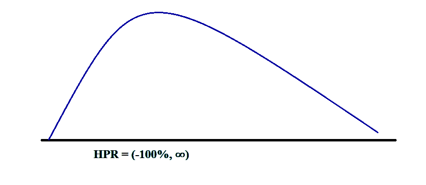
c.  Some of the important features of lognormal distribution are:

i.  It is bounded by 0 on the lower end.

ii.  The upper end of this distribution is unbounded.

iii.  This distribution is skewed to the right (i.e. it is positively skewed).

d.  A lognormal distribution can be drawn on the graph as follows:

Lognormal Distribution Quantitative Methods CFA level 1 Study Notes

e.  If V0 is the beginning value of the distribution and Vt is the ending value of the distribution, then its ratio is such that:

Lognormal Distribution Quantitative Methods CFA level 1 Study Notes

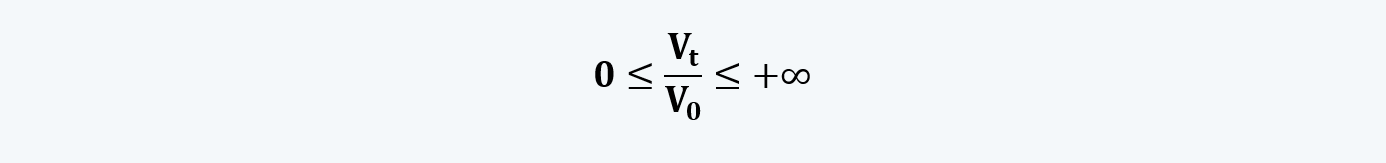
f.  This ratio i.e. Vt / V0  is distributed lognormally. However, its natural log, i.e. IN (Vt / V0), is normally distributed and unbounded at both ends. It is used as an approximation of actual returns.

g.  The log of the ratio of the ending and beginning value of the distribution also equals the log of one plus the holding period returns.

Lognormal Distribution Quantitative Methods CFA level 1 Study Notes

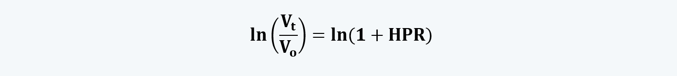
h.  The key point to be noted here is that if an asset’s continuously compounded return is normally distributed, then the asset’s future price must be lognormally distributed.

i.  Thus, we can say that:

Lognormal Distribution Quantitative Methods CFA level 1 Study Notes

This was calculated by taking the natural log of:

Lognormal Distribution Quantitative Methods CFA level 1 Study Notes

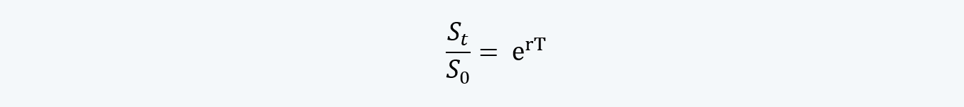
Thus, we can also say that:

Lognormal Distribution Quantitative Methods CFA level 1 Study Notes

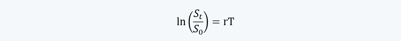
j.  We can express the term St / S0 as follows:

Lognormal Distribution Quantitative Methods CFA level 1 Study Notes

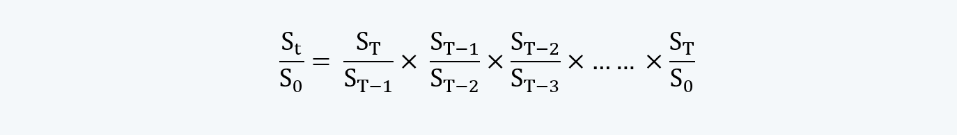
Thus we can also write the equation as follows:

Lognormal Distribution Quantitative Methods CFA level 1 Study Notes

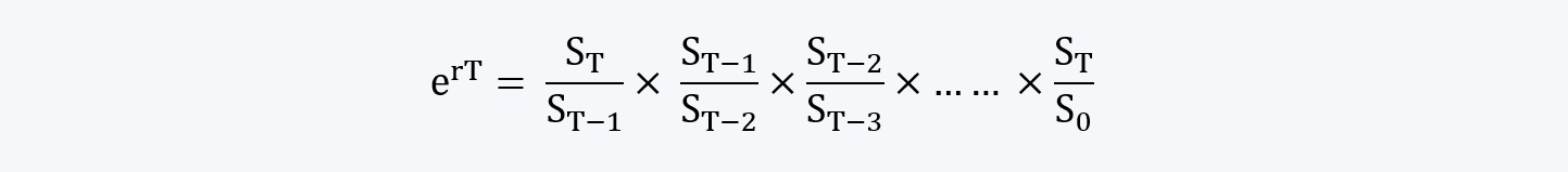
If we take the log of the above equation:

Lognormal Distribution Quantitative Methods CFA level 1 Study Notes

We can see that the above equation is now a linear combination of independent-randomly distributed variables. Therefore, a lognormal distribution is a normal one.

k.  For the normal distribution to be useful in the analysis, there are two conditions that need to be satisfied:

i.  Independence: It means that each of the individual variables in the distribution should be completely independent and should not have any information with respect to the other variables. The variables should be so unrelated so that:

Lognormal Distribution Quantitative Methods CFA level 1 Study Notes

That is, the probability of event ‘T’, given that the event ‘T-1’ has already happened, equals the probability of event ‘T’. This means that the previous event does not affect the probability of the following event.

ii.  Identically Distributed: This means that all the variables must be identically distributed. This requirement emphasizes the stationarity of the data, i.e. the mean and the standard deviation of the data should not change from observation to observation.

However, the mean and standard deviations may not be the same for different financial and economic conditions.

These conditions imply:

Lognormal Distribution Quantitative Methods CFA level 1 Study Notes

Which is equal to:

Lognormal Distribution Quantitative Methods CFA level 1 Study Notes

l.  A lognormal distribution can be applied to the volatility, which is the standard deviation of the continuously compounded returns.