LOS B, C, D, and E require us to:

b.  distinguish between one-tailed and two-tailed tests of hypotheses,

c.  explain a test statistic, Type I and Type II errors, a significance level, and how significance levels are used in hypothesis testing,

d.  explain a decision rule, the power of a test, and the relation between confidence intervals and hypothesis tests,

e.  distinguish between a statistical result and an economically meaningful result 

The details of the steps involved in hypothesis testing are:

1.  State The Hypothesis

a.  There are basically two hypotheses that are required to be tested, i.e. null hypothesis and the alternative hypothesis.

b.  Null Hypothesis, denoted by H₀:

i.  It is the statement that we are testing.

ii.  It is usually the hypothesis that we are interested in rejecting.

iii.  A null hypothesis can be built in three ways, i.e.:

Where, θ is the population mean and θ₀ is the hypothesized value of the population mean.

c.  An alternative hypothesis, denoted by H_a:

i.  It is the statement that we are trying to validate.

ii.  It can be built in three ways:

d.  The different possibilities represented by the two hypotheses should be mutually exclusive and collectively exhaustive.

e.  Hypothesis tests generally concern the true value of a population parameter as determined using a sample statistic.

f.  The main purpose of hypothesis testing is to estimate the likelihood that the sample statistics accurately represent the population parameters. This can be done using the one-tailed and two-tailed tests.

1.1.  One-Tailed Hypothesis

a.  One-tailed tests are comparisons based on a single side of the distribution.

b.  There could be two types of one-tailed hypothesis, i.e. right-tailed hypothesis and left-tailed hypothesis.

c.  The right-tailed hypothesis test for the values of the population parameters which are lower than or equal to the sample statistics.

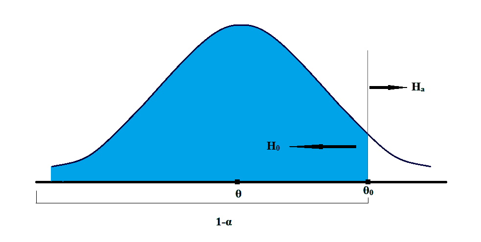
Here, it is believed that the parameter is bigger than the hypothesized value of the mean. In this test, everything at the left of the hypothesized mean is the null hypothesis, which is to be rejected. Whereas, everything to the right is the alternative hypothesis.

The equations for the right-tailed hypothesis can be written as:

d.  The left-tailed hypothesis test for the values of the population parameters higher than or equal to the sample statistics.

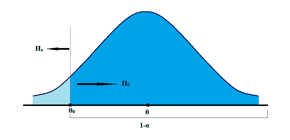Here, it is believed that the parameter is smaller than the hypothesized value of the mean. In this test, everything to the right of the hypothesized mean is the null hypothesis, which is to be rejected. Whereas, everything to the left is the alternative hypothesis.

The equations for the right-tailed hypothesis can be written as:

1.2.  Two-Tailed Hypothesis

a.  In contrast to the one-tailed test, two-tailed tests admit the possibility of the true population parameter lying in either tail of the distribution.

b.  As per this test, we reject the null in favor of the alternative if the evidence indicates that the population parameter is either smaller or larger than θ₀.

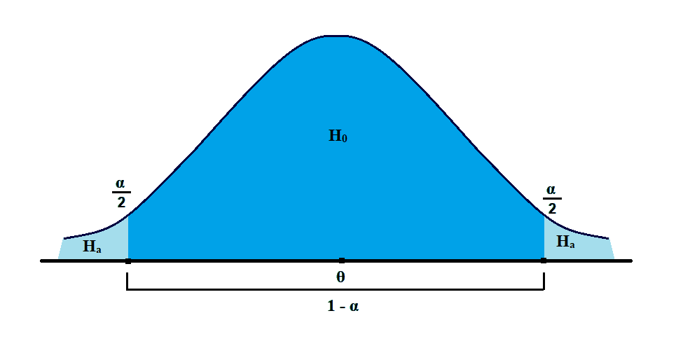
c.  Here, in the two-tailed test, we have to see if the parameter is not equal to the hypothesized value.

d.  The equations for the two-tailed hypothesis can be written as:

NOTE:

In all the cases, H₀ is conducted at the point of equality, i.e. H₀: µ = µ₀.

2.  Choosing the Appropriate Test and Its Probability Distribution

a.  The selection of an appropriate null hypothesis and, as a result, an alternative hypothesis, centers around economic or financial theory as it relates to the point estimate(s) being tested.

b.  Two-tailed tests are more “conservative” than one-tailed tests. In other words, they lead to a fail-to-reject the null hypothesis conclusion more often.

c.  One-tailed tests are often used when financial or economic theory proposes a relationship of a specific direction.

d.  If we look at the hypothesis for testing, such as:

They are always stated as inequality and tested as equality.

e.  The test statistic is a calculated quantity based on a sample whose value is the basis for acceptance and rejection of the null hypothesis.

The test statistic can be calculated by reducing the hypothesized statistic from the sample statistic and dividing the result by the standard error. That is,

Or,

Here, the sample statistic (i.e. ) is the representative of the population parameter (i.e. µ₀).

f.  For example, consider the following hypothesis:

The null hypothesis says that the mean of the sample statistic is less than or equal to the population parameter; whereas, for the alternative hypothesis, it should be greater. For this hypothesis we could have one of the three outcomes as follows:

i.  If, the mean is equal to the hypothesized value, i.e. x̄ = μ₀, the value of x̄ – μ₀ = 0; and thus, the test statistic will also be 0. The only way to reject the null hypothesis would be if we have the value of α = 0.

ii.  If the mean is less than the hypothesized value, i.e. x̄ < μ₀, the value of x̄ – μ₀ < 0; and thus, the test statistic will also be negative. Here also we cannot reject the null hypothesis as the value of the test statistic is not positive.

iii.  If the mean is higher than the hypothesized value, i.e. x̄ > μ₀, the value of x̄ – μ₀ > 0; and thus, the test statistic will also be positive. This is the only way to reject the null hypothesis.

g.  The question that now arises is what the value of the test statistic should be so as to accept or reject the null hypothesis? It depends upon the test that is used to test the hypothesis.

h.  Test statistics that we implement will generally follow one of the following distributions:

i.  t-distribution (it requires t-test)

ii.  Standard normal (it requires z-test)

iii.  F-distribution (it requires F-test)

iv.  Chi-square distribution (it requires chi-square test)

3.  Specifying the Significance Levels

a.  Before we discuss the significance levels that should be selected, we need to understand the conditions under which the null hypothesis is accepted or rejected and the errors that may be there resultantly:

Type I errors occur when we reject a null hypothesis that is actually true. Type II errors occur when we do not reject a null hypothesis that is false.

Thus, the mutually exclusively problems are:

i.  If we mistakenly reject the null, we make a Type I error.

ii.  If we mistakenly fail to reject the null, we make a Type II error.

iii.  Because we can’t reject and fail to reject simultaneously because of the mutually exclusive nature of the null and alternative hypothesis, the errors are also mutually exclusive.

The rate at which we correctly reject a false null hypothesis is known as the power of the test.

b.  The level of significance is the desired standard of proof against which we measure the evidence contained in the test statistic.

i.  The level of significance is identical to the level of a Type I error and, like the level of a Type I error, is often referred to as “alpha,” or a.

ii.  How much sample evidence do we require to reject the null? It is a statistical “burden of proof.”

iii.  The level of confidence in the statistical results is directly related to the significance level of the test and, thus, to the probability of a Type I error.

c.  Reducing the probability of type I errors involves reducing the α, but doing so increases the probability of type II errors. Thus, the only way to decrease the probability of both errors at the same time is to increase the sample size because such an increase reduces the denominator of our test statistic.

d.  The test is considered more powerful if it correctly accepts or rejects the null hypothesis. And, to make a test more powerful, when more than one test statistic is available, use the one with the highest power for the specified level of significance. The bigger the sample size, the better are the results.

4.  State The Decision Rule

a.  The decision rule uses the significance level and the probability distribution of the test statistic to determine the value above (below) which the null hypothesis is rejected.

b.  The critical value (CV) of the test statistic is the value above (below) which the null hypothesis is rejected. It is also known as the rejection point.

i.  For one-tailed tests, it is indicated with a subscript α.

ii.  For two-tailed tests, it is indicated with a subscript α/2.

c.  So the decision rule for the three types of hypothesis testing, i.e. right-tailed test, left-tailed test, and two-tailed tests are:

i.  For the right-tailed test, we will reject the null hypothesis if the test statistic is greater than the critical value.

ii.  For the left-tailed test, we will reject the null hypothesis if the test statistic is less than the critical value.

iii.  For the two-tailed test, we will reject the null hypothesis if the absolute value of the test statistic is greater than the absolute value of the critical value.

5.  Collect The Data & Calculate The Test Statistics

The quality of test results to a large extent depends upon the quality of data collected. In practice, data collection is likely to represent the largest portion of the time spent in hypothesis testing, and care should be given to the sampling considerations, particularly biases introduced in the data collection process. One should avoid measurement errors and time period bias as well.

6.  Make the Statistical Decision

The statistical process is completed when we compare the test statistic from Step 5 with the critical value in Step 4 and assess the statistical significance of the result. The decision involves a rejection of or failure to reject the null hypothesis.

7.  Make The Economic Decision

a.  One of the end purposes of hypothesis testing is to make the economic decision in a scientific manner. The economic or investment decision should take into account not only the statistical evidence but also the economic value of acting on the statistical conclusion

b.  If we recall, the value of the test statistics is:

Here, with an increase in the sample size (i.e. n), the test statistic also increases.

Therefore, small departures from µ₀ may prove to be statistically significant, but may not be economically significant, as it involves transaction cost taxes and risk. We may find strong statistical evidence of a difference but the only weak economic benefit to acting.

c.  Because the statistical process often focuses only on one attribute of the data, other attributes may affect the economic value of acting on our statistical evidence. Thus, a statistically significant difference in mean return for two alternative investment strategies may not lead to economic gain if the higher-returning strategy has much higher transaction costs.