LOS C, D, E, and F require us to:

c.  calculate and interpret the effective annual rate, given the stated annual interest rate and the frequency of compounding;
d.  solve time value of money problems for different frequencies of compounding;
e.  calculate and interpret the future value (FV) and present value (PV) of a single sum of money, an ordinary annuity, an annuity due, perpetuity (PV only), and a series of unequal cash flows;
f.  demonstrate the use of a time line in modeling and solving the time value of money problems.

In this section, we discuss the following:

a.  Present Value (PV) of an investment, or the initial investment;

b.  Future Value (FV) of an investment;

c.  N, i.e. the number of compounding periods or the time for which the investment is held; and

d.  The rate of interest (r), which is usually the discounting rate, or the expected return on investment.

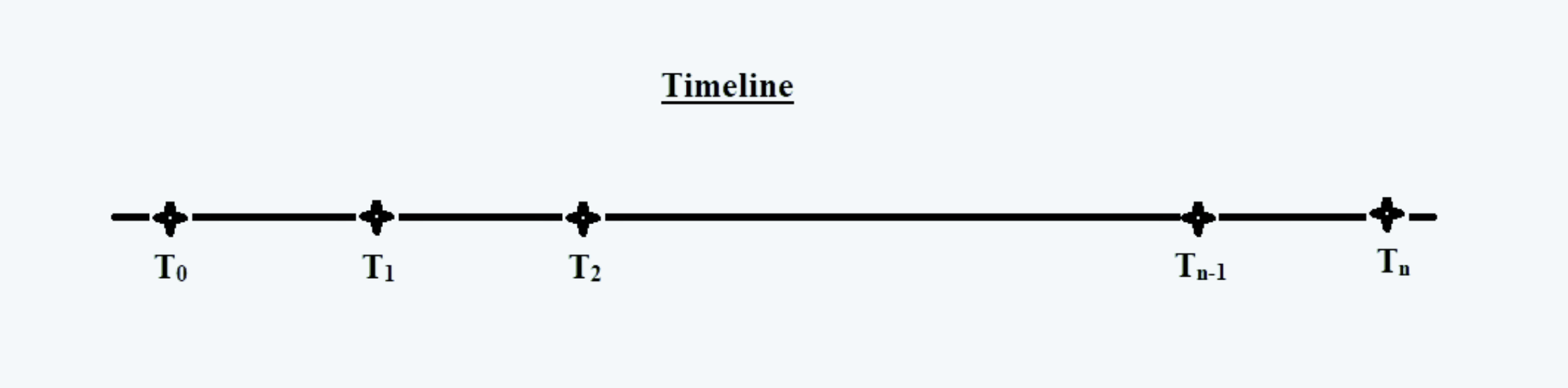
Consider the following timeline:

Now, if $ 100 was invested today, the total amount that would be received one year hence (assuming a rate of interest of 5%) would be: $ 105 [i.e. 100*(1+0.05)]:

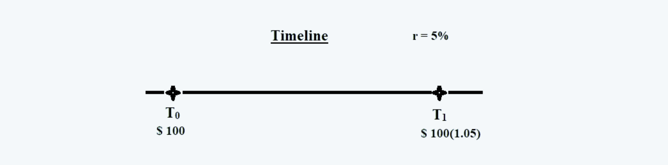
And the value at the beginning of year one would be $ 105. In year 2, a further interest would be earned on this $ 105 and be compounded. Thus, the value of the investment at the end of year 2 would be $110.25 [i.e. 105*(1.05)].

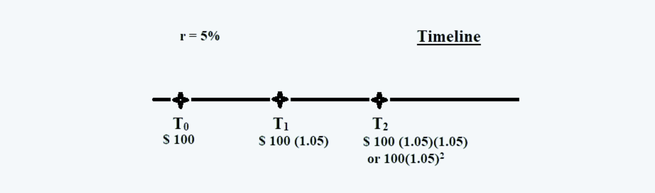
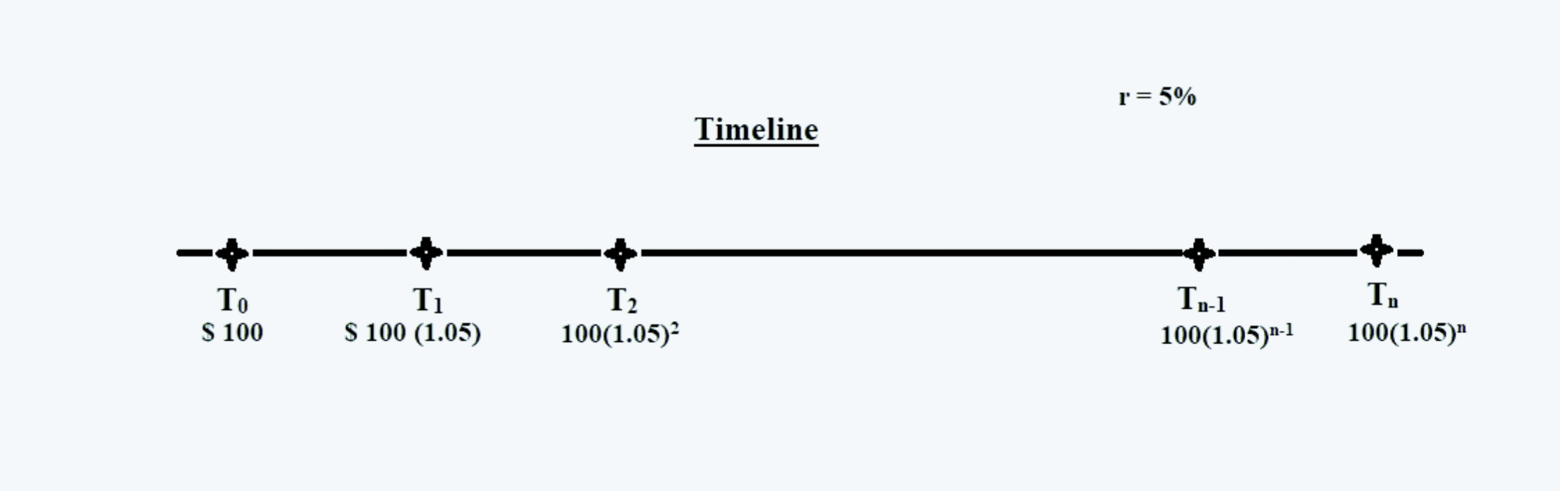
Similarly, for the time period of n, the future value of the $100 investment would be $ 100*(1.05)ⁿ:

1.  Basic Formula for Present & Future Value

Thus we can sum up the effect of compounding and relation between the interest and time as follows:

For discounting the future value of cash flow to arrive at the present value, the following formula can be used:

2.  Multiple Compounding

While using the above-mentioned formulas, the values of ‘r’ and ‘N’ must be compatible with the time. For example, if an amount of $200 is compounded at 4% for the next five years, we would use the following values for compounding:

Therefore, the future value of a cash flow at the interest rate of r, for N-years, compounded m-times a year would be:

And the present value would be:

3.  Continuous Compounding

When there is a continuous compounding of the interest rates, the future value of the amount invested today at an interest rate of ‘r’ for a time period of ‘N’ would be:

 And the present value of the future stream of cash flow is:

4.  Effective Annual Rates

When there is a compounding of interest multiple times in a year, would yield an absolute return of more than what is earned if it was compounded once annually. For example, $ 100 invested at 4% for a year would yield:

It can thus be seen from the above example that the effective interest rates keep on increasing as the number of times it compounded increases.

So, the effective annual rate can be calculated using the following formula:

And, when there is a continuous compounding, the effective interest rate can be calculated using the following formula:

So, if we know the effective annual rate, we can also find the stated rate as follows:

And, if the interest is compounded continuously, the stated interest would be calculated as follows:

5.  Annuity

a.  An annuity is a finite set of equal sequential cash flows.

b.  There are two types of annuities: an ordinary annuity and the annuity due.

c.  An ordinary annuity is one that is payable at the end of each equal sequential period.

For example, consider the following timeline:

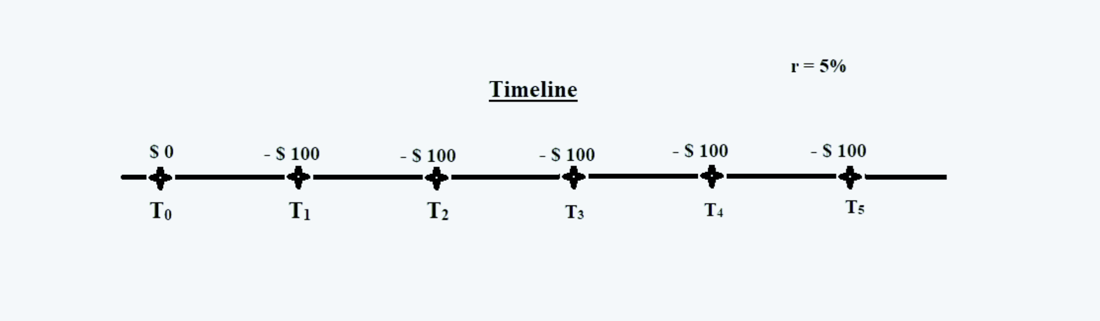
In the above timeline, since the payment begins at the end of the current time period i.e. T₀, therefore it is an ordinary annuity. Also, all the payments are equal and sequential, for a finite period of 5 years.

So the time period, payment, their respective future value, and total future value of the annuity at the end of the year 5 are:

Calculating the future value using the above procedure, i.e. calculating the future value of the individual payment and then summing it up is a very long and tedious task, especially if the number of payments is large. Alternatively, the future value of an ordinary annuity can be calculated using the following formula:

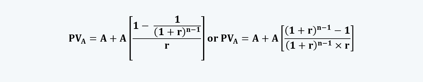
On similar lines, as discussed above, we can also find the present value of an ordinary annuity using the formula:

d.  Whereas, an annuity due is the one that is payable at the beginning of each period.

For example, consider the following timeline:

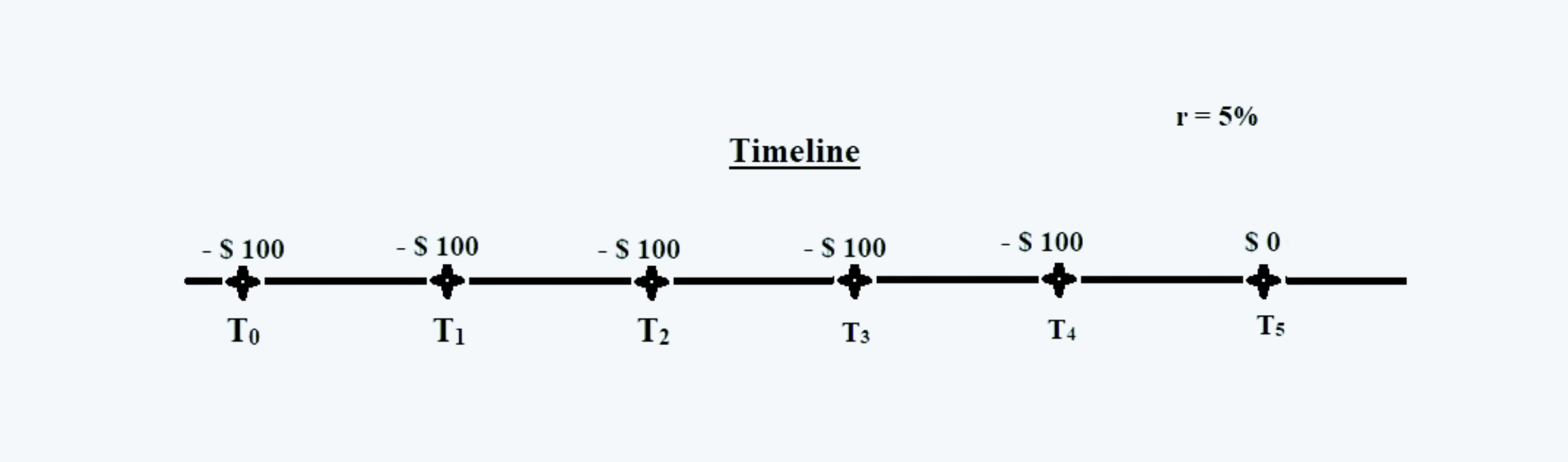
In the above timeline, since the payment begins at the beginning of the current time period i.e. T₀, therefore it is an annuity due. Also, all the payments are equal and sequential, for a finite period of 5 years.

So the time period, payment, their respective future value, and total future value of the annuity at the end of the year 5 are:

Calculating the future value using the above procedure, i.e. calculating the future value of the individual payment and then summing it up is a very long and tedious task, especially if the number of payments is large. Alternatively, the future value of an annuity due can be calculated using the following formula:

Also, the formula for the present value of an annuity due is:

If we notice the above-mentioned formulas for the present value of the annuities, they are nothing but the future value discounted back to the present date at the applicable discount rate, or:

6.  Unequal Cash Flows

Consider the following timeline:

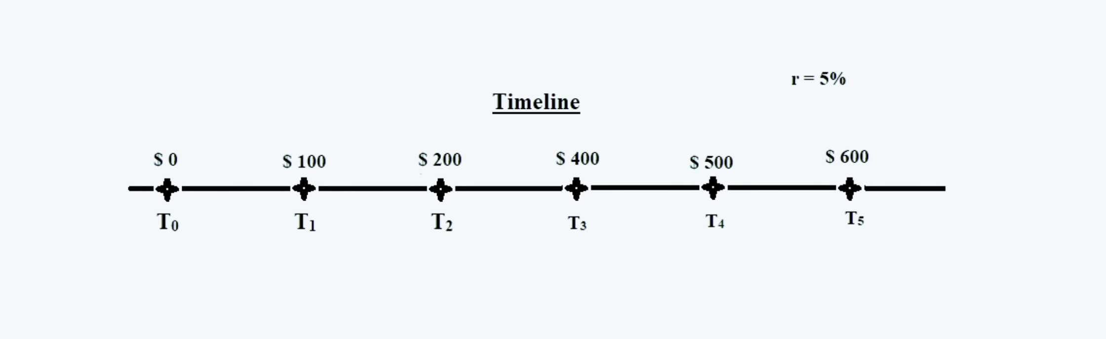
The time period, payment, their respective future value, and total future value of the payment series at the end of year 5 are:

7.  Perpetuity

a.  Perpetuity is nothing but an annuity with an infinite holding period, i.e. N= ∞.

b.  Thus, perpetuity must have:

i.  leveled or equal cash flows,

ii.  sequential payments, and

iii.  infinite holding period.

c.  Now, consider the formula for calculation of the present value of an annuity, which is:

For perpetuity, since N  → ∞,

                                  1/ (1+ r)ⁿ  → 0

Therefore, the present value of a perpetuity is:

For example, there is the perpetuity of $ 100 per annum at the interest rate of 5%, its present value at the beginning would be:

Now, consider there is the perpetuity of $ 100 at the interest rate of 5% starting 5 years from today, then its present value at the end of 5 years from now would be:

Now we can calculate its present value, today, by discounting this value at 5% for 5 years, as follows:

8.  Solving for Rate of Interest / Time Period / Payment

a.  If we are given the price today (i.e. PV) for an amount receivable N years from now (i.e. FV), we can calculate the rate of interest as follows:

We know that:

Thus,

Or,

b.  Similarly, we can also find the value of N, as follows:

Given the equation:

Thus,

So we can find the value of N as follows:

For example: For how many years should an amount of $100 be invested so that it doubles, at the interest rate of 7%?

We are given:        FV = $200

                              PV = $100             

                              r = 7%

And we need to solve for N.

As per the above formula,

Or, it takes 10.2448 years for the money to double at the interest rate of 7%.

c.  We can calculate the annual payments that should be made so that it has a certain present value if we are given the interest rates and the time horizon.

We know that the present value of an annuity is:

Solving for A in the above equation:

This formula is mostly useful in calculating the EMIs and the series of annual payments.

For example:

We purchased an asset worth $ 100,000 on an installment basis to be paid in the next 5 years beginning at the end of the current year. The applicable interest rate is 5%. We have to find a number of equal installments that should be paid for the next 5 years.

or,