Course Content
THE TIME VALUE OF MONEY
This chapter is covered in reading 6 of study session 2 of the material provided by the institute. After reading this chapter, a student should be able to: a) interpret interest rates as required rates of return, discount rates, or opportunity costs; b) explain an interest rate as the sum of a real risk-free rate and premiums that compensate investors for bearing distinct types of risk; c) calculate and interpret the effective annual rate, given the stated annual interest rate and the frequency of compounding; d) solve time value of money problems for different frequencies of compounding; e) calculate and interpret the future value (FV) and present value (PV) of a single sum of money, an ordinary annuity, an annuity due, perpetuity (PV only), and a series of unequal cash flows; f) demonstrate the use of a timeline in modeling and solving time value of money problems.
0/2
STATISTICAL CONCEPTS AND MARKET RETURNS
This chapter is covered in reading 7 of study session 2 of the material provided by the Institute. After reading this chapter, a student should be able to: a. distinguish between descriptive statistics and inferential statistics, between a population and a sample, and among the types of measurement scales; b. define a parameter, a sample statistic, and a frequency distribution; c. calculate and interpret relative frequencies and cumulative relative frequencies, given a frequency distribution; d. describe the properties of a data set presented as a histogram or a frequency polygon; e. calculate and interpret measures of central tendency, including the population mean, the sample mean, arithmetic mean, weighted average or mean, geometric mean, harmonic mean, median, and mode; f. calculate and interpret quartiles, quintiles, deciles, and percentiles; g. calculate and interpret 1) a range and a mean absolute deviation and 2) the variance and standard deviation of a population and of a sample; h. calculate and interpret the proportion of observations falling within a specified number of standard deviations of the mean using Chebyshev’s inequality; i. calculate and interpret the coefficient of variation and the Sharpe ratio; j. explain skewness and the meaning of a positively or negatively skewed return distribution; k. describe the relative locations of the mean, median, and mode for a unimodal, nonsymmetrical distribution; l. explain measures of sample skewness and kurtosis; m. compare the use of arithmetic and geometric means when analyzing investment returns.
0/9
PROBABILITY CONCEPTS
This chapter is covered in reading 8 of study session 2 of the material provided by the Institute. After reading this chapter, a student should be able to: a. define a random variable, an outcome, an event, mutually exclusive events, and exhaustive events; b. state the two defining properties of probability and distinguish among empirical, subjective, and a priori probabilities; c. state the probability of an event in terms of odds for and against the event; d. distinguish between unconditional and conditional probabilities; e. explain the multiplication, addition, and total probability rules; f. calculate and interpret 1) the joint probability of two events, 2) the probability that at least one of two events will occur, given the probability of each and the joint probability of the two events, and 3) a joint probability of any number of independent events; g. distinguish between dependent and independent events; h. calculate and interpret an unconditional probability using the total probability rule; i. explain the use of conditional expectation in investment applications; j. explain the use of a tree diagram to represent an investment problem; k. calculate and interpret covariance and correlation; l. calculate and interpret the expected value, variance, and standard deviation of a random variable and of returns on a portfolio; m. calculate and interpret covariance given a joint probability function; n. calculate and interpret an updated probability using Bayes’ formula; o. identify the most appropriate method to solve a particular counting problem and solve counting problems using factorial, combination, and permutation concepts.
0/9
COMMON PROBABILITY DISTRIBUTIONS
This chapter is covered under reading 9, study session 3, as provided by the institute. After reading this chapter, a student shall be able to: a. define a probability distribution and distinguish between discrete and continuous random variables and their probability functions; b. describe the set of possible outcomes of a specified discrete random variable; c. interpret a cumulative distribution function; d. calculate and interpret probabilities for a random variable, given its cumulative distribution function; e. define a discrete uniform random variable, a Bernoulli random variable, and a binomial random variable; f. calculate and interpret probabilities given the discrete uniform and the binomial distribution functions; g. construct a binomial tree to describe stock price movement; h. calculate and interpret tracking error; i. define the continuous uniform distribution and calculate and interpret probabilities, given a continuous uniform distribution; j. explain the key properties of the normal distribution; k. distinguish between a univariate and a multivariate distribution and explain the role of correlation in the multivariate normal distribution; l. determine the probability that a normally distributed random variable lies inside a given interval; m. define the standard normal distribution, explain how to standardize a random variable, and calculate and interpret probabilities using the standard normal distribution; n. define shortfall risk, calculate the safety-first ratio, and select an optimal portfolio using Roy’s safety-first criterion; o. explain the relationship between normal and lognormal distributions and why the lognormal distribution is used to model asset prices; p. distinguish between discretely and continuously compounded rates of return and calculate and interpret a continuously compounded rate of return, given a specific holding period return; q. explain Monte Carlo simulation and describe its applications and limitations; r. compare Monte Carlo simulation and historical simulation.
0/6
SAMPLING AND ESTIMATION
This chapter is covered under reading 10, study session 3, as provided by the institute. After reading this chapter, a student shall be able to: a. define simple random sampling and a sampling distribution; b. explain sampling error; c. distinguish between simple random and stratified random sampling; d. distinguish between time-series and cross-sectional data; e. explain the central limit theorem and its importance; f. calculate and interpret the standard error of the sample mean; g. identify and describe desirable properties of an estimator; h. distinguish between a point estimate and a confidence interval estimate of a population parameter; i. describe properties of Student’s t-distribution and calculate and interpret its degrees of freedom; j. calculate and interpret a confidence interval for a population mean, given a normal distribution with 1) a known population variance, 2) an unknown population variance, or 3) an unknown variance and a large sample size; k. describe the issues regarding selection of the appropriate sample size, data mining bias, sample selection bias, survivorship bias, look-ahead bias, and time-period bias.
0/7
HYPOTHESIS TESTING
This chapter is covered under reading 11, study session 3, as provided by the institute. After reading this chapter, a student shall be able to: a. define a hypothesis, describe the steps of hypothesis testing, and describe and interpret the choice of the null and alternative hypotheses; b. distinguish between one-tailed and two-tailed tests of hypotheses; c. explain a test statistic, Type I and Type II errors, a significance level, and how significance levels are used in hypothesis testing; d. explain a decision rule, the power of a test, and the relation between confidence intervals and hypothesis tests; e. distinguish between a statistical result and an economically meaningful result; f. explain and interpret the p-value as it relates to hypothesis testing; g. identify the appropriate test statistic and interpret the results for a hypothesis test concerning the population mean of both large and small samples when the population is normally or approximately normally distributed and the variance is 1) known or 2) unknown; h. identify the appropriate test statistic and interpret the results for a hypothesis test concerning the equality of the population means of two at least approximately normally distributed populations, based on independent random samples with 1) equal or 2) unequal assumed variances; i. identify the appropriate test statistic and interpret the results for a hypothesis test concerning the mean difference of two normally distributed populations; j. identify the appropriate test statistic and interpret the results for a hypothesis test concerning 1) the variance of a normally distributed population, and 2) the equality of the variances of two normally distributed populations based on two independent random samples; k. formulate a test of the hypothesis that the population correlation coefficient equals zero and determine whether the hypothesis is rejected at a given level of significance; l. distinguish between parametric and nonparametric tests and describe situations in which the use of nonparametric tests may be appropriate.
0/8
Quantitative Methods
About Lesson

LOS G requires us to:

identify and describe desirable properties of an estimator


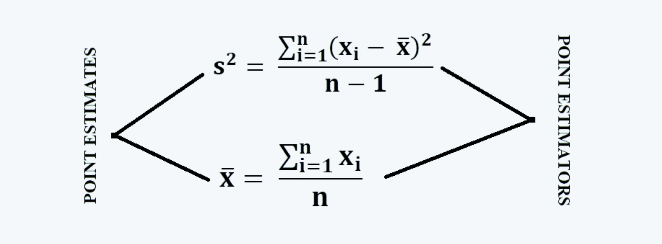
a.  When we take samples from the population, we calculate its mean and the variance. These are the values at a single point, and thus the point estimates. And, the formulas used in the calculation of these estimates are the estimators.

b.  Estimators are the generalized mathematical expressions for the calculation of sample statistics, and an estimate is a specific outcome of one estimate.

c.  Estimates take on a single numerical value and are, therefore, referred to as point estimates. It is a fixed number specific to that sample. It has no sampling distribution.

point estimates and estimators Quantitative Methods CFA level 1 Study Notes

d.  The point estimators should have certain desirable properties, they are:

i.  Unbiased: An estimator is considered unbiased when the estimated expected value calculated using the estimator is equal to the value of the parameter being estimated.
For example, the value of the sample mean and variance must equal the value of the mean and the variance of the population. That is,

desirable properties of point estimators Quantitative Methods CFA level 1 Study Notes

Where n is the sample size and m is the number of samples.
And,

desirable properties of point estimators Quantitative Methods CFA level 1 Study Notes
Note, that here we use n-1 instead of n because, if we had used n as the denominator instead, it would have produced a consistently smaller variance, hence creating biasedness.

ii.  Efficiency: An estimator is said to be efficient when no other estimator has a smaller variance.

Consider the following figure, for example:

Efficiency of estimators Quantitative Methods CFA level 1 Study Notes

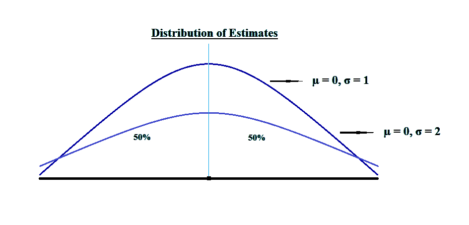
In the above figure, the distribution with a higher graph has a lower standard deviation, therefore, it makes a better estimate.

iii.  Consistency: An estimator is considered more consistent when the probability of obtaining estimates close to the value of the population parameter increases as the sample size increases. Consistency is asymptotic in nature, thereby requiring a large number of observations.

Thus, for an estimator to be consistent,

desirable properties of point estimators Quantitative Methods CFA level 1 Study Notes