LOS D requires us to:

distinguish between unconditional and conditional probabilities

1.  Unconditional Probabilities

a.  The unconditional probability is the independent probability of a single outcome resulting from the possibility of space.

b.  It is calculated based on the empirical evidence, by dividing the observations of the desired outcome by the probability space of all outcomes.

c.  For example, if an investment manager expects the return on investment to be higher than the risk-free rate. And it was observed that out of 1000 observations regarding the returns obtained by the portfolio managers, 800 were above the risk-free rate. Then, the unconditional probability of a manager earning more than risk-free rates based on the empirical observations would be 0.8 (i.e. 800/1000).

2.  Conditional Probability

a.  Conditional probability is the probability of an event if another event says B has already happened.

b.  Conditional probability is also calculated based on the empirical evidence, by dividing the observations of the desired outcome by the probability space of the observation, given the condition of event B has already occurred.

c.  For example, if an investment manager expects the return on investment to be higher than the risk-free rate, given that he has already earned a return greater than 0. And it was observed that out of 1000 observations regarding the returns obtained by the portfolio managers, 900 had already earned a return greater than 0, and 800 were above the risk-free rate. Then, the conditional probability of a manager earning more than risk-free rates, given that he has already earned a positive return, based on the empirical observations would be 0.889 (i.e. 800/900).

Note: Here the denominator is not the entire space of total outcomes. Rather, it is the space of event B. This can be graphically presented as follows:

d.  We can write the equation of the conditional probability with a formal notation as follows:

We can also re-arrange this equation to write:

We can depict the probabilities of two events occurring together as follows:

e.  That was how we calculate the probability of the two events occurring together; on similar lines, we can also calculate the probability of either of the two events.

The equation for calculating the probabilities of event A or B is:

Graphically it can be presented as follows:

3.  Independent Events

a.  Independent events are those events where the occurrence of one event does not have any impact on the occurrence of the other event.

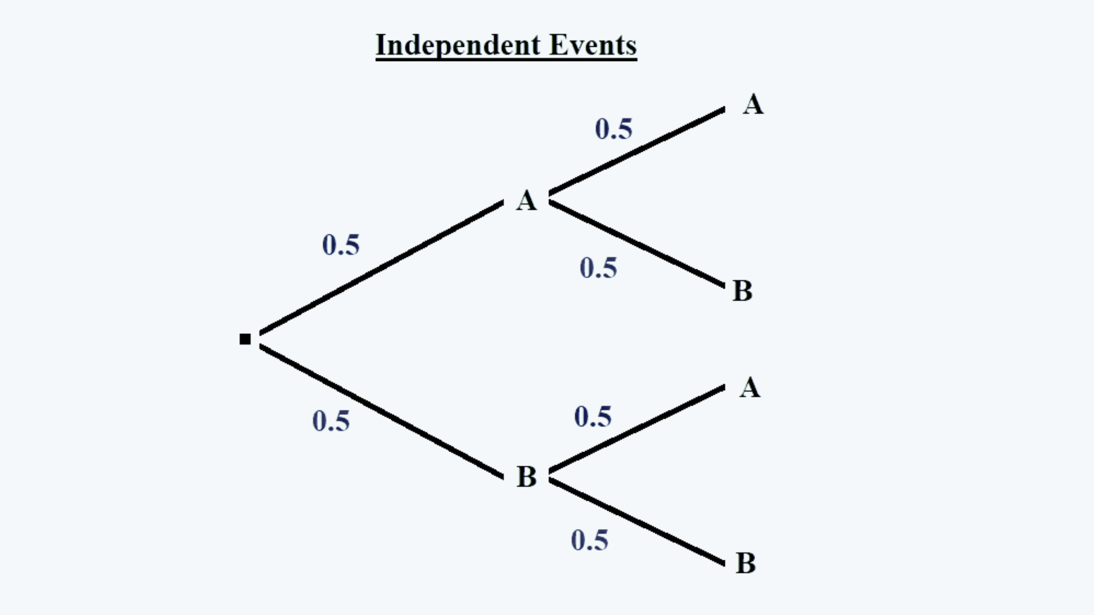
b.  For example, a student appeared in an exam that is conducted in two parts A and B, having objective-type questions with two options as the probable answer. Since the student didn’t know the answers to any of the questions and there was no negative marking either; so he circled the first option for each answer. Now there is a 50% probability of clearing either part of the exam. Also as per the rules, he would be declared ‘passed’ only in either of the two parts only.

Now, say P(A) is the probability of clearing the first part of the exam, and P(B), the probability of clearing the second par. And, if the student appears again for the same exam, unprepared, then also the result would not be affected by the fact that he cleared either part in the previous attempt or not.

Here there is no relation between clearing both the attempts, and both are independent events. Thus the probability of B given that A has already happened is equal to the probability of B only. And the joint probability of both events is also the product of the two probabilities.

This can be better explained in the form of the following tree structure:

c.  Thus, we can say that the following equations hold true for independent events:

And,