LOS E requires us to:
describe common technical analysis indicators (price-based, momentum oscillators, sentiment, and flow of funds)
a. The technical analyst uses a variety of technical indicators to supplement the information gleaned from charts.
b. A technical indicator is any measure based on price, market sentiment, or fund flows that can be used to predict price changes. These indicators measure how potential changes in supply and demand might affect a security’s price.
1. Price Based Indicators
a. Price-based indicators incorporate information contained in the current and past history of market prices. Indicators of this type range from simple (e.g., a moving average) to complex (e.g., a stochastic oscillator).
b. Some of the important price-based indicators are:
1.1. Moving Averages
a. A moving average is the average of the closing price of a security over a specified number of periods.
b. Moving averages smooth out short-term price fluctuations, giving the technician a clearer image of the market
c. Moving averages may range from fast-moving to slow-moving depending upon the number of calculation days, such as 9, 20, 50, 100, 200, etc.
d. There are different types of moving averages. They are:
1.1.1. Simple Moving Average (SMA)
a. A simple moving average is easy to construct and widely used by technical analysts.
b. To construct a moving average the time span of the average has to be first determined. 30-day moving average averages out fluctuations occurring over all the possible 30-day time span over the periods under observation.
c. To construct a 100-day SMA for instance:
i. The prices are observed over the first 100-days are summed up and divided by 100 to obtain a simple average.
ii. This is the first value of constructing a 100-day SMA.
iii. To obtain the next value, the price prevailing on the first day is excluded, while including the price on the 101st
iv. This represents the next 100-day period.
v. The average of these observations is the next value of 100-day SMA.
vi. This process is repeated for the time period, one intends to cover.
d. The choice of time period is very important in constructing the moving averages. If the prices move in cycles, say over 2 years, a 750-day moving average will smoothen out all intermediate trends. A 10-day moving average will represent many minor fluctuations present on the timeline and would be of little use in determining the tops and bottoms of a trend.
e. The lesser the time span, the more sensitive is the moving average and vice-versa. Therefore, a moving average should provide an optimum trade-off between oversensitivity and delay in identifying the reversals.
1.1.2. Exponential Moving Averages (EMA)
a. A simple moving average constructed over a long time span generally lags the price trend. Therefore, EMA provides a shortcut method of weightings. This method also provides more weight to the recent data.
b. An example of a 50-day moving chart is as follows:
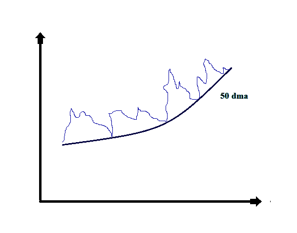
In the above example, the moving average line smoothen outs the minor fluctuations in the actual price data and shows the trends in the movement of prices. The moving average trend line also acts as a support line for the actual price data.
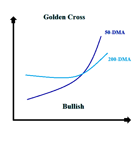
c. The moving averages across different time spans could be used to analyze the indicators, Such as:
i. If the moving average of lesser time-span (say 50-day) crosses the moving average of a higher time span (say 200-day) from below, then it is considered as a ‘golden cross’ and a bullish market may be expected.
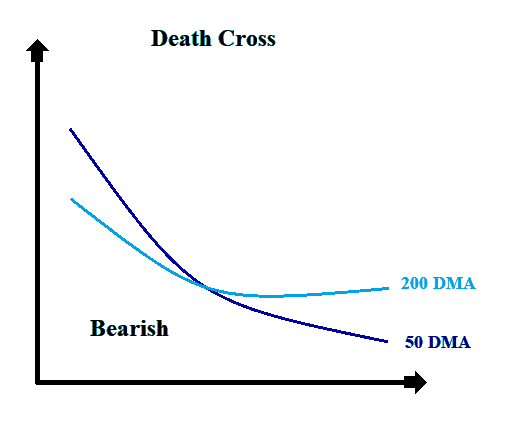
ii. If the moving average of lesser time-span (say 50-day) crosses the moving average of a higher time span (say 200-day) from above, then it is considered as a ‘death cross’ and a bearish market may be expected.
1.2. Bollinger Bands
a. Bollinger bands are good indicators of the volatility of the stocks.
b. They can be formed by taking a moving average and adding and reducing the standard deviation from the same. This gives us a range within which the prices are moving.
c. An example of the Bollinger band is:
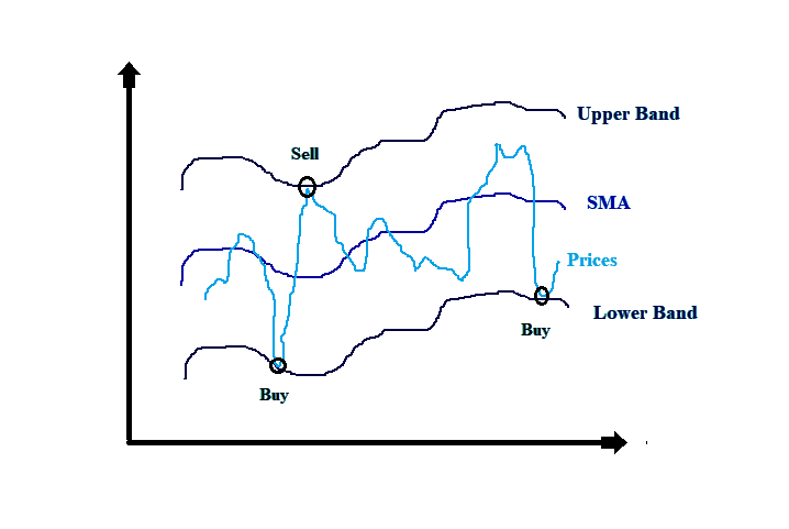
More the volatility of the security, wider is the bands.
d. When the price touches the upper band, it is an indicator that the securities can be sold. Whereas, the prices touching the lower band gives a buy signal.
2. Momentum Oscillators
a. One of the key challenges in using indicators overlaid on a price chart is the difficulty of discerning changes in market sentiment that are out of the ordinary. Momentum oscillators are intended to alleviate this problem. They are constructed from price data, but they are calculated so that they either oscillate between a high and low (typically 0 and 100) or oscillate around a number (such as 0 or 100). Because of this construction, extreme highs or lows are easily discernible.
b. These extremes can be viewed as graphic representations of market sentiment when selling or buying activity is more aggressive than historically typical.
c. Because they are price-based, momentum oscillators also can be analyzed by using the same tools technicians use to analyze prices, such as the concepts of the trend, support, and resistance.
d. Some of the important momentum oscillators are:
2.1. Rate of Change (ROC) Oscillator
a. One of the simplest and widely used methods to measure momentum is to compute the rate at which the price of a stock, or market index, changes over a certain period of time. The ROC index is constructed to measure such price changes.
b. If the ROC index is to be constructed for measuring a 50-day rate of change in prices; the price prevailing on a certain day is compared to the price 50 days earlier. The resulting ratio is the ROC Index value for that day.
c. The formula for calculating the ROC oscillator is: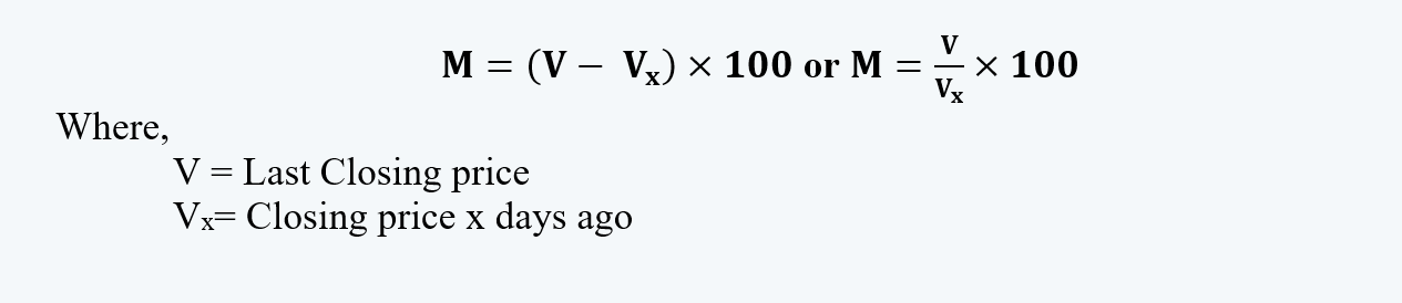
d. A rising ROC index indicates growth in momentum (a bullish factor) and a falling index a loss in momentum (a bearish factor).
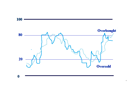
2.2. Relative Strength Index (RSI)
a. RSI is another oscillator that measures momentum.
b. As opposed to the other measures, this indicator measures the relative internal strength of a stock or market against itself.
c. The formula for calculating the RSI is as follows:
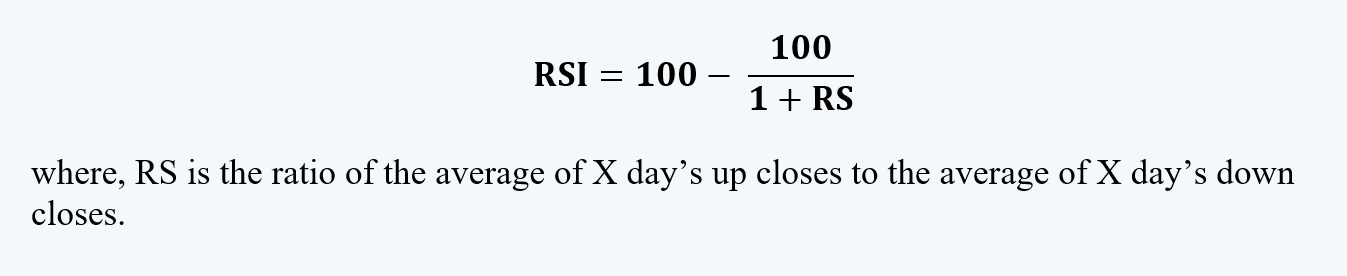
d. From the formula, it is evident that the value of the RSI indicator fluctuates between 0 and 100.
e. A graph is plotted using the RSI values. On this graph, the oversold and overbought positions are drawn at 30 and 70 levels on a scale of 0 to 100.
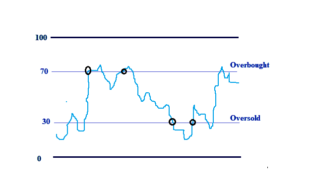 When the indicator crosses the oversold or overbought position, it is a warning signal to the trader. At this stage, it presents an opportunity to the trader to consider either buying or selling.
i. When the indicator crosses, the oversold position at 30 from above, it signals that one should sell the stock.
ii. While, at the same position if the indicator crosses from below, it is taken as a signal for buying.
iii. At the overbought position at 70, the opposite holds true.
2.3. Stochastic Oscillators
a. The stochastic oscillator is based on the observation that in uptrends, prices tend to close at or near the high end of their recent range, and in downtrends, they tend to close near the low end. The logic behind these patterns is that if the shares of a stock are constantly being bid up during the day but then lose value by the close, the continuation of the rally is doubtful. If sellers have enough supply to overwhelm buyers, the rally is suspect. If a stock rallies during the day and is able to hold on to some or most of those gains by the close, that sign is bullish.
b. The formula to calculate the stochastic oscillator is (The oscillator is composed of two lines, called %K and %D, that are calculated) as follows:
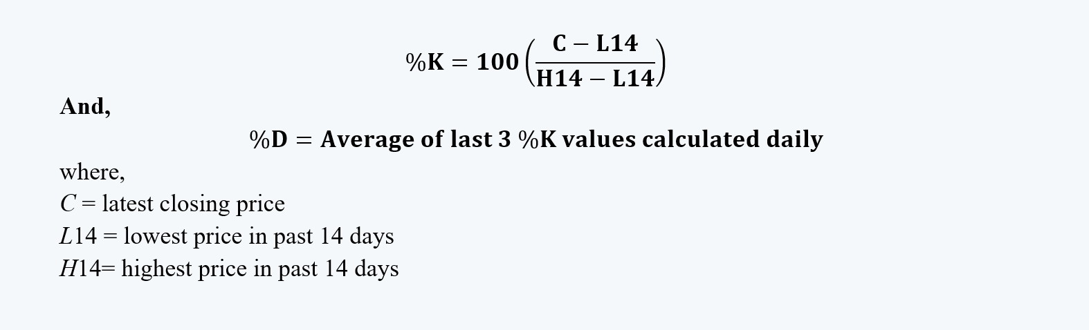
c. The stochastic oscillator oscillates between 0 and 100 and has a default setting of a 14-day period, which, again, might be adjusted to the situation.
d. When this oscillator is used with other indicators that give the same signal, it means convergence, else it is divergence.
2.4. Moving Average Convergence / Divergence
a. MACD like ROC is an oscillator that measures momentum.
b. It is called so, as it continuously converges and diverges away from the horizontal reference line.
c. It is constructed by taking the difference or the ratio of the short-term and long-term moving average. The points obtained are plotted against a reference line or a signal line. The reference lines represent the points where the two EMAs have identical values.
d. We can also impose a third EMA or a moving average obtained from the oscillator itself. This is the ‘signal line’ as it acts as a trigger that alerts the trader to take appropriate buy or sell decisions.
e. From the movement of the MACD indicator, it can be known, whether the shorter-term moving average is below or above the longer-term moving average.
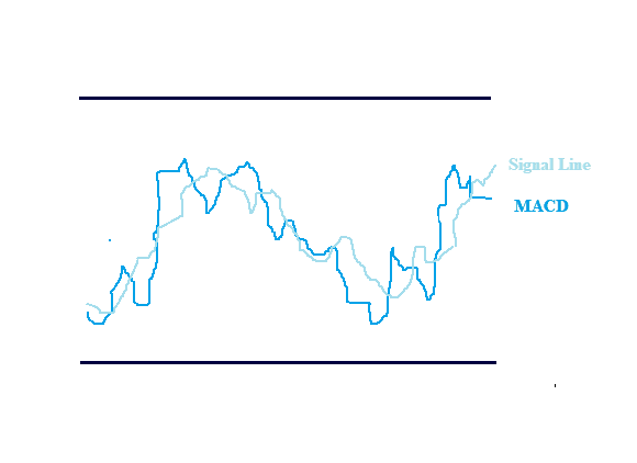
f. The point of crossing between the MACD and reference line act as the signals to buy and sell.
i. When the MACD line crosses the signal line from below, it is an indicator for buying the stock.
ii. Whereas, where it crosses the signal line from above, it is an indicator to sell.
3. Sentiment Indicators
a. Sentiment indicators attempt to gauge investor activity for signs of increasing bullishness or bearishness. Sentiment indicators come in two forms—investor polls and calculated statistical indices.
3.1. Opinion Polls
a. A wide range of services conducts periodic polls of either individual investors or investment professionals to gauge their sentiment about the equity market.
b. Some of the most common opinion polls conducted are:
i. Investors Intelligence Advisor’s Sentiments Report
ii. Market Vane Bullish Consensus
iii. Consensus Bullish Sentiment Index
iv. Daily Sentiment Index
c. There are also reports by the American Association of Individual Investors (AAII), which polls individual investors.
3.2. Calculated Statistical Indices
a. The other category of sentiment indicators is indicators that are calculated from market data, such as security prices.
b. The two most commonly used are derived from the options market; they are the put/call ratio and the volatility index. Additionally, many analysts look at margin debt and short interest.
c. The put-call ratio is calculated by dividing the number of put options trading by the number of call options trading for a particular financial instrument.
Investors who buy put options on security are presumably bearish, and investors who buy call options are presumably bullish. The volume in call options is greater than the volume traded input options over time, so the put/call ratio is normally below 1.0.
d. The CBOE Volatility Index (VIX) is a measure of near-term market volatility calculated by the Chicago Board Options Exchange. Since 2003, it has been calculated from option prices on the stocks in the S&P 500. The VIX rises when market participants become fearful of an impending market decline. These participants then bid up the price of puts, and the result is an increase in the VIX level. Technicians use the VIX in conjunction with the trend, pattern, or oscillator tools, and it is interpreted from a contrarian perspective. When other indicators suggest that the market is oversold and the VIX is at an extreme high, this combination is considered bullish
e. Investor psychology plays an important role in the intuition behind margin debt as an indicator. When stock margin debt is increasing, investors are aggressively buying and stock prices will move higher because of increased demand. Eventually, the margin traders use all of their available credit, so their buying power (and, therefore, demand) decreases, which fuels a price decline. Falling prices may trigger margin calls and forced selling, thereby driving prices even lower.
f. The short interest ratio represents the number of day trading activities represented by short interest. To facilitate comparisons of large and small companies, common practice is to “normalize” this value by dividing short interest by average daily trading volume to get the short-interest ratio:

It is considered to show market sentiment and to be a contrarian indicator. Some people believe that if a large number of shares are sold short and the short-interest ratio is high, the market should expect a falling price for the shares because of so much negative sentiment about them.
4. Flow of Funds Indicators
a. Technicians look at fund flows as a way to gauge the potential supply and demand for equities.
b. Demand can come in the form of margin borrowing against current holdings or cash holdings by mutual funds and other groups that are normally large holders of equities, such as insurance companies and pension funds. The more cash these groups hold, the more bullish is the indication for equities.
c. One caveat in looking at potential sources of demand is that, although these data indicate the potential buying power of various large investor groups, the data say nothing about the likelihood that the groups will buy.
d. On the supply side, technicians look at a new or secondary issuance of stock because these activities put more securities into the market and increase supply.
e. Different types of flow-of-funds indicators are:
4.1. Arms Index (TRIN)
a. A common flow of funds indicator is the Arms Index, also called the TRIN (for “short-term trading index”).
b. This indicator is applied to a broad market (such as the S&P 500) to measure the relative extent to which money is moving into or out of rising and declining stocks.
c. The index is a ratio of two ratios:

d. When this index is near 1.0, the market is in balance; that is, as much money is moving into rising stocks as into declining stocks. A value above 1.0 means that there is more volume in declining stocks; a value below 1.0 means that most trading activity is on rising stocks.
4.2. Margin Debt
Margin debt was previously discussed as an indicator of market sentiment. Margin debt is also widely used as a flow-of-funds indicator because margin loans may increase the purchases of stocks and declining margin balances may force the selling of stocks.
4.3. Mutual Fund Cash Position
a. An analyst’s initial intuition might be that when mutual fund cash positions are relatively low, fund managers are bullish and anticipate rising prices but when fund managers are bearish, they conserve cash to wait for lower prices.
b. Advocates of this technical indicator argue exactly the opposite: When the mutual fund cash position is low, fund managers have already bought, and the effects of their purchases are already reflected in security prices.
c. However, when the cash position is high, that money represents buying power that will move prices higher when the money is used to add positions to the portfolio.
d. The mutual fund cash position is another example of a contrarian indicator. Some analysts modify the value of the cash percentage to account for differences in the level of interest rates.
e. When interest rates are low, holding cash can be a substantial drag on the fund’s performance if the broad market advances. When interest rates are high, holding cash is less costly.
4.4. New Equity Issuance and Secondary Offerings
a. When a company’s owners decide to take a company public and offer shares for sale, the owners want to put those shares on the market at a time when investors are eager to buy. That is, the owners want to offer the shares when they can sell them at a premium price. Premium prices occur near market tops. The new equity issuance indicator suggests that as the number of initial public offerings (IPOs) increases, the upward price trend may be about to turn down.
b. Technicians also monitor secondary offerings to gauge potential changes in the supply of equities. Although secondary offerings do not increase the supply of shares, because existing shares are sold by insiders to the general public, they do increase the supply available for trading or the float. So, from a market perspective, secondary offerings of shares have the potential to change the supply-and-demand equation as much as IPOs do.