LOS B requires us to:

explain the capital allocation line (CAL) and the capital market line (CML)

1.  Capital Allocation Line

Consider the following figure:

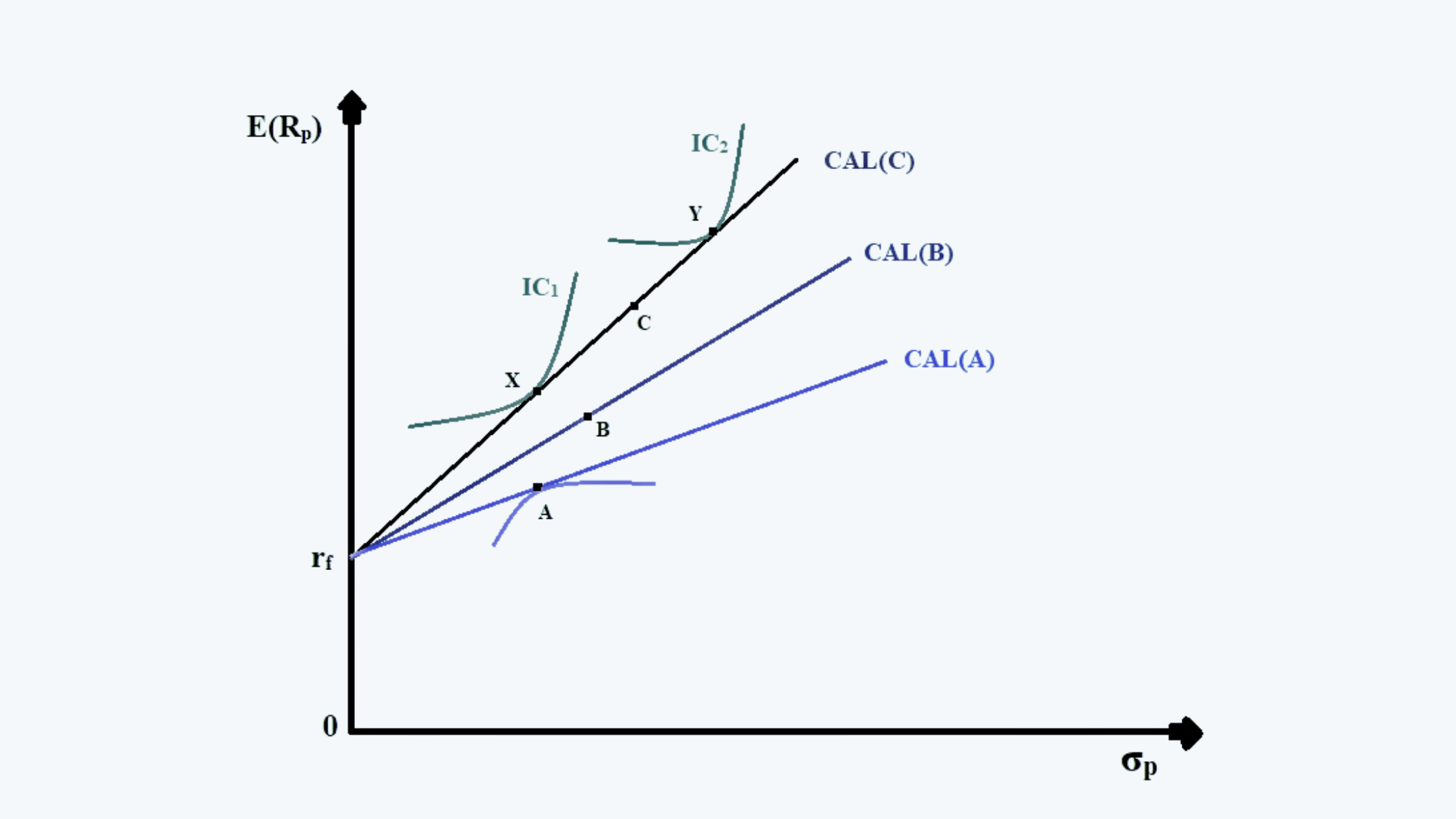
In the above figure,

a.  CAL(A), CAL(B), and CAL(C) represent the capital allocation line for the three assets A, B, and C. Points A, B, and C are the risk-return points if 100% allocation were made in the respective assets. All these points lie on their respective Markowitz Efficient Frontier.

b.  To recall from the previous chapter, the equations of the capital allocation line is:

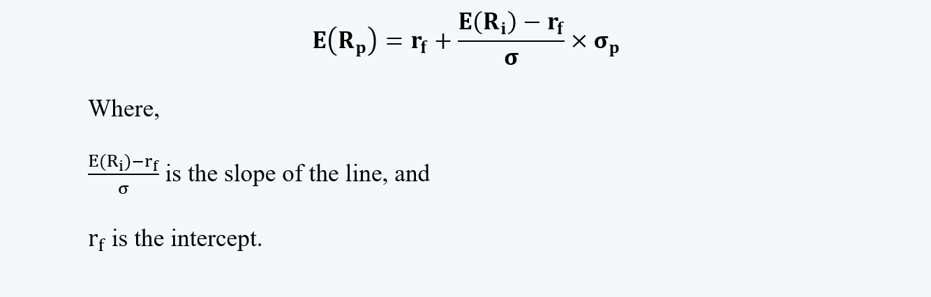
c.  Though points B and C provide a better return in comparison to point A, it carries higher risk as well. And all these points are efficient portfolios on their respective minimum variance curves.

d.  In a choice between the three allocation lines, it is best to choose the one with the highest slope (like CAL(C) in this case). This is mainly because the line with the higher slope always has a point corresponding to the point on the lower line, with the same level of risk but a higher return. Just like in the above figure, X and A have almost the same level of risks but X has a higher return. And despite, this point being unattainable, it can be attained through lending/borrowing.

e.  Now suppose there are two investors one risk-averse and the other, a risk seeker, with their respective highest attainable indifference curves, IC₁ and IC₂. These investors should make the investment up to point X and Y respectively. These are the points at which the indifference curves are tangent to the highest possible capital allocation line, i.e. CAL(C). Thus they are the most efficient and desirable asset allocation points.

f.  Point X can be attained by combining the risky asset portfolio of C and lending at the risk-free rate. And point Y can be attained by borrowing.

There are certain assumptions behind the above optimal portfolio theory. They are:

a.  There exists homogeneity of expectations of investors. That is, this theory assumes that all the investors have the same economic expectation regarding the risk-return distribution of each asset. Therefore there is only one optimal risky portfolio.
If the expectations were not homogeneous, there would have been multiple optimal risky portfolios.

b.  This theory assumes that the markets are informationally efficient. There is no excess return to the active investors.
If the markets were not informationally efficient, the active investors may have earned excess returns.

2. Capital Market Line

a.  A market usually includes all the assets that are investible and tradable. In order to keep it simple to understand, we limit the markets to the major equity indices of the country.

b.  The capital market line or CML is a CAL where the risky portfolio is the market portfolio.

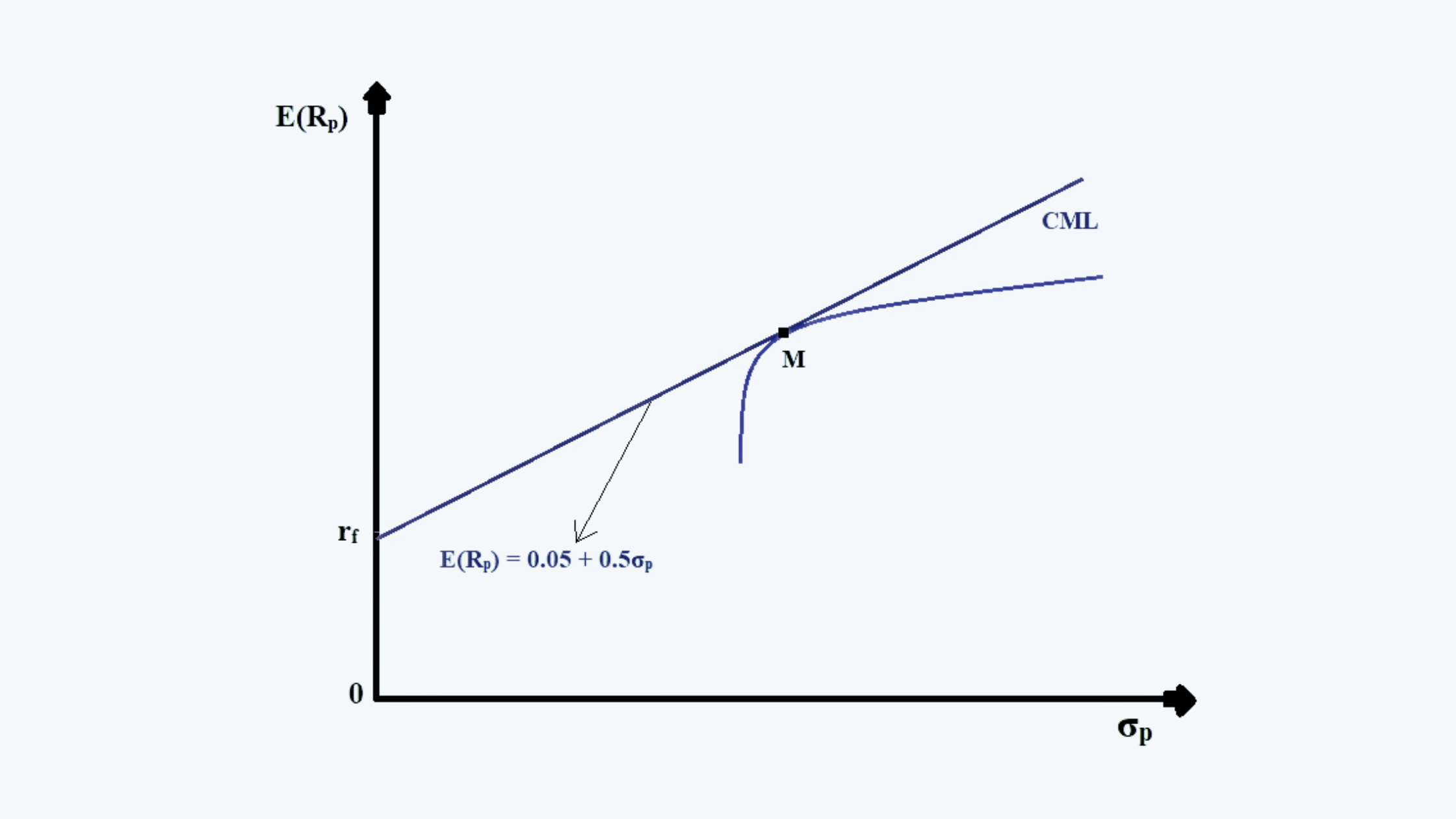
c.  We can draw a CML, similar to a CAL as follows:

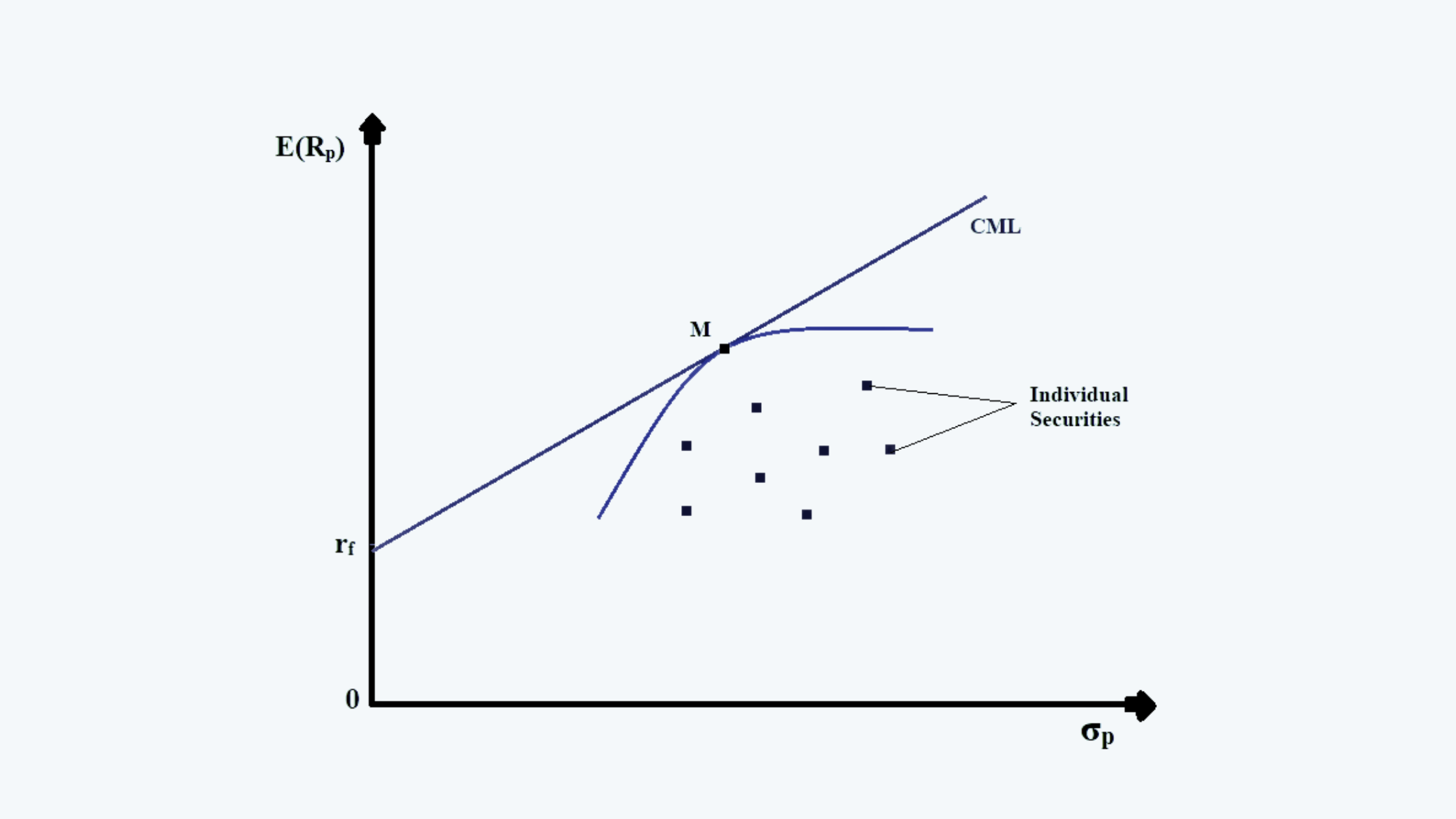
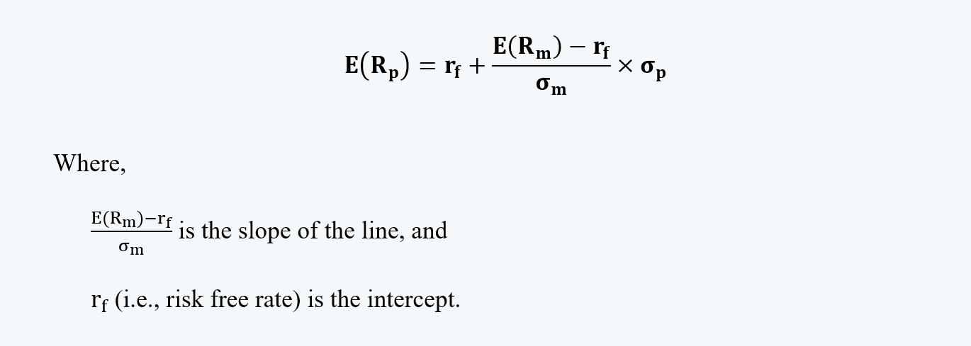
d.  In the above figure, CML is the capital market line. The equation of the line is:

3.  Example

Consider a market with an expected return of 15% and a standard deviation of 20%. Assuming the risk-free rate of 5%, the slope of the CML would be:

 This means that every one unit change in the standard deviation of the portfolio changes the return also by 0.5 units on the CML.

The equation of the CML would thus be:

E(R_p) = 0.05 + 0.5σ_p

We can now calculate the different levels of return and risk for different weights of the risk-free asset and the market portfolio, as follows:

We can draw this on a graph as follows:

We can now create a leveraged portfolio by borrowing at a risk-free rate using the leverage of 25%, 50%, and 100%. So the weights, return, and risk of each portfolio would be as follows:

We can plot this on the above graph as follows:

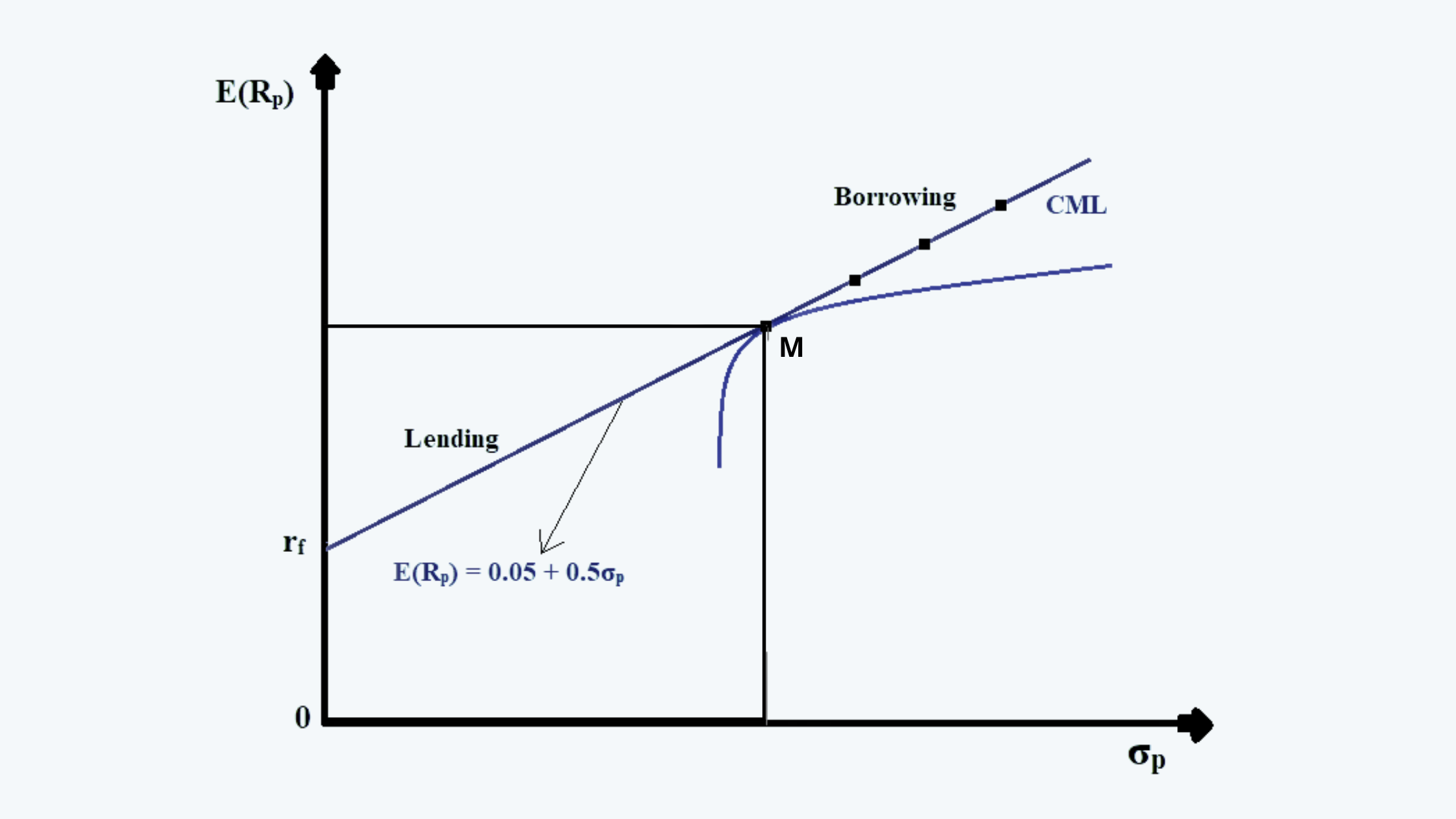
These points for the borrowing portfolio lie above point M. They sure do offer a higher return, but also carry higher risk.

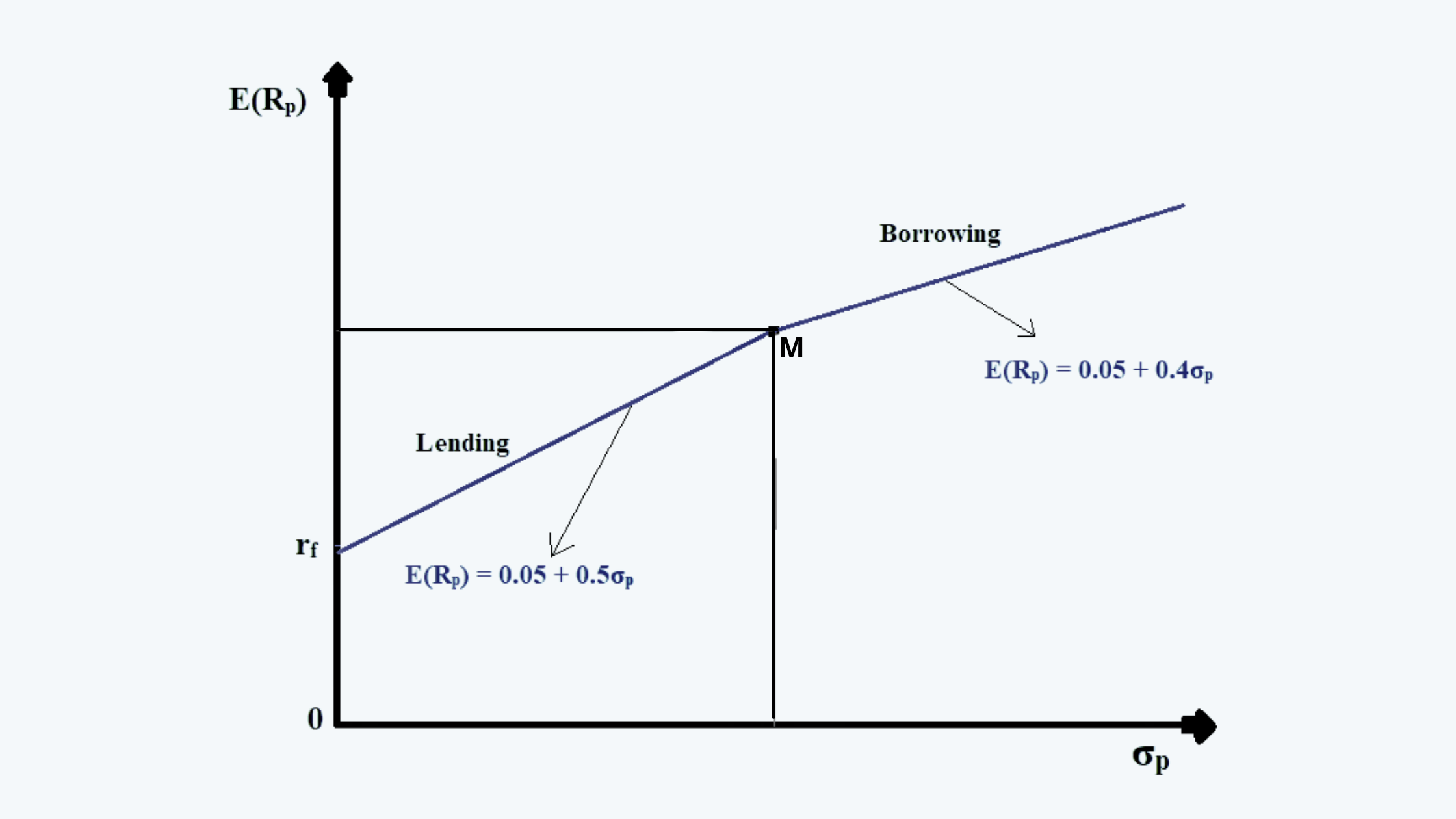
Now suppose that the investor can borrow at the rate of 7% and lend at the risk-free rate. This will result in the change in slope of the CML from point M. The slope of the line beyond point M would be:

And the equation of the line beyond that point would be:

E(R_p) = 0.05 + 0.4σ_p

We can represent this on a graph as follows:

So, if we were to borrow 75% of the funds at the rate of 7%:

i.  Weight, W₁ would be -0.75;

ii.  Weight W₂ would be 1.75

iii.  The expected return on the portfolio would be:

E(R_p) = (-0.75)(0.07) + (1.75)(0.15) = 21%

iv.  And, the portfolio risk would be:

 σ_p = (1.75) (0.20) = 35%

Thus in comparison to the borrowing at the risk-free rate, the returns on this portfolio have decreased, but the risk remains the same.