LOS H and I require us to:

h.  describe and interpret the minimum-variance and efficient frontiers of risky assets and the global minimum-variance portfolio.
i.  explain the selection of an optimal portfolio, given an investor’s utility (or risk aversion) and the capital allocation line.

Consider the following figure:

In the above figure:

a.  The straight line DE, with ρ = 1, shows the change in the risk-return pattern of the portfolio at different levels of weights of each asset. Since there is a perfect correlation between the assets, it is a straight line, indicating that as there is an increase in the weight of the asset with the higher return in the portfolio, the portfolio returns also increase; but there is a corresponding increase in the risk as well.

b.  However, when there is less than perfect correlation, i.e. ρ < 1, we get a curved risk-return line. As shown in the above figure, when we move upwards from point E towards D, initially there is an increase in return along with a decrease in risk. This pattern can be observed up to point Z; beyond which the increase in return is only accompanied by the increase in risk as well.

c.  Thus, while moving from point E towards D, that is increasing the proportion of asset B in the portfolio, the investor would not want to settle at any point before Z, such as point C, because increasing the weight of the asset B would move the investor towards a more optimal point, with maximum return and minimum risk. Point Z is thus the ‘global optimal point’.

d.  Thus the curved line DE with a correlation less than 1 is called the ‘minimum variance frontier’. And the intercept ZD on the curve DE represents the ‘Markowitz Efficient Frontier’.

1.  Adding Risk-Free Asset

Consider the minimum variance frontier we derived above. Now let us add a risk-free asset to the portfolio, as below:

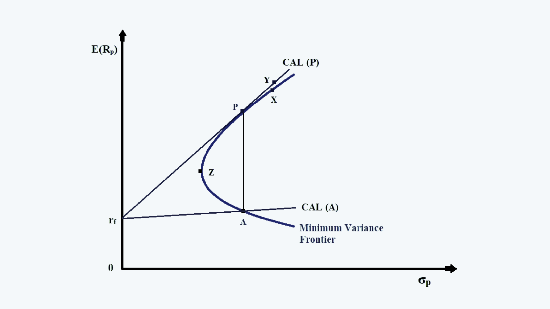
a.  CAL(A) shows the capital allocation line of asset A, whereas the line CAL(P) shows the capital allocation line of the portfolio after adding the risk-free asset.

b.  Any point on CAL (A) is less efficient than CAL (P), because of corresponding to that point, there is another point on CAL (P), which offers better return (E(R_p)) at the given level of risk (σ_p).

c.  Thus, in the above figure, we can see that point P dominates point A, as it offers higher returns. Similarly, point Y dominates point X. Point Y can be achieved by leveraging the portfolio.

2.  Two-Fund Separation Theorem

a.  According to this theorem, all the investors, regardless of taste, risk preferences, or wealth, will hold a combination of two portfolios, a risk-free asset, and a risky portfolio.

b.  Thus the investment decision can be taken by:

     i.  Identifying the optimal risky portfolio with regards to the investor preferences,

    ii.  Prepare a capital allocation line which is a linear combination of the risk-free assets and risky assets.

   iii.  The optimal risky portfolio is the point at which the CAL is tangent to the Markowitz Efficient Frontier, i.e. point P in the above figure.

   iv.  The final financing decision depends upon the risk tolerance level of the investor.

    v.  If the investor is risk-averse, he could choose to be at any point on the CAL below the point P on the above figure. This he can do by lending the money at a risk-free rate.

   vi.  If the investor is risk-neutral, he would rather choose to be at point P.

  vii.  If the investor is a risk-seeker, then he can borrow money to invest in the risky portfolio, to be at any point on the CAL above point P.