LOS H to L requires us to:
h. define the continuous uniform distribution and calculate and interpret probabilities, given a continuous uniform distribution;
i. explain the key properties of the normal distribution;
j. distinguish between a univariate and a multivariate distribution and explain the role of correlation in the multivariate normal distribution;
k. determine the probability that a normally distributed random variable lies inside a given interval;
l. define the standard normal distribution, explain how to standardize a random variable, and calculate and interpret probabilities using the standard normal distribution;
1. Continuous Uniform Variables
a. It is the simplest continuous probability distribution; it is very similar to the discrete uniform distribution, except for a little difference.
b. The continuous uniform distribution is described by a lower limit ‘a’ and an upper limit ‘b’. These are also called the ‘parameters of the distribution’.
c. We can draw the probabilities of a continuous uniform distribution as follows:
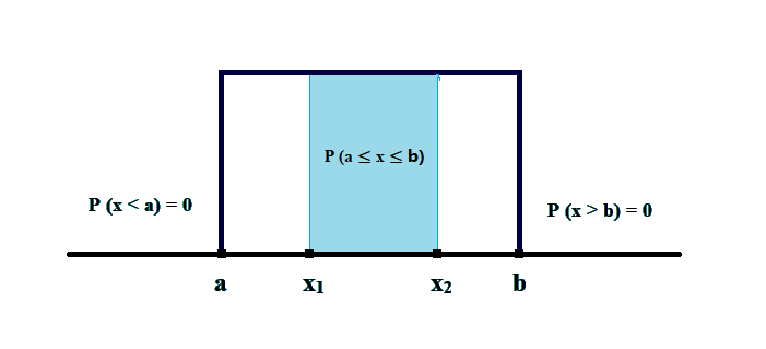
In the above diagram:
i. All the probabilities are uniformly distributed between ‘a’ and ‘b’, such that P (a ≤ x ≤ b) = 100%.

ii. The probability of anything less than ‘a’ and greater than ‘b’ is zero; i.e.

iii. The probabilities of any variables lying in a range between ‘a’ and ‘b’, say ‘x1’and ‘x2’ can be calculated as follows:

d. We can draw the cumulative distribution function for continuous uniform probabilities as follows:
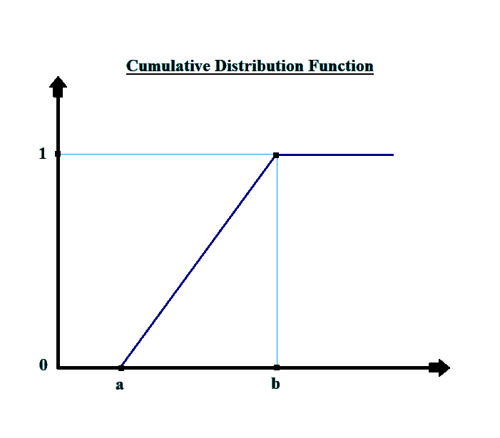
In this figure:
i. The cumulative probabilities of the distribution are zero up to point ‘a’.
ii. The cumulative probability increases in a linear fashion after point ‘a’ up to point ‘b’, when it becomes equal to one. This increase is linear because the probabilities are uniformly distributed.
iii. Beyond point ‘b’ it remains constant at one. This is mainly because the cumulative probabilities up to point ‘b’ reach one and do not increase post that.
e. The probability density function (pdf) for a uniform random variable is:

Thus if the value of ‘a’ is 0 and that of ‘b’ is 8 then the function of ‘x’ is f(x) = 1/(8-0) = 0.125 for values of ‘x’ between ‘a’ and ‘b’.
f. The cumulative distribution function, which is denoted by F(x) can be written as:

g. The mean of a continuous uniform function is:

h. The variance of a continuous uniform function is:

2. Normal Distribution
a. A normal distribution is a non-uniform continuous distribution.
b. The central limit theorem states that the sum of a large number of independent random variables is approximately normally distributed.
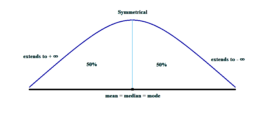
c. A normal distribution curve is a bell-shaped curve, divided into two symmetrical halves. A normal distribution curve is such that it covers information about 100% of the observed data.
The median of a normal distribution equals its mean and mode and its tails extend towards infinity on both sides. It can be drawn as follows:
 d. The properties of a normal distribution are as follows:
i. A normal distribution is completely described by the mean (µ) and variance (σ2).

ii. The curve is neither positively skewed nor negatively skewed; the skewness of a normal distribution curve is zero, such that:

iii. The kurtosis of a normal distribution curve is 3.
iv. A linear combination of normally distributed variables is also normally distributed, i.e.

Or, if the return on individual assets is normally distributed for all assets in a portfolio, then the return on the portfolio is also normally distributed.
2.1. Univariate Distribution
a. A univariate distribution describes the distribution of a single random variable.
b. It is measured by two variables, i.e. mean and variance.
2.2. Multivariate Distribution
a. A multivariate distribution specifies the probabilities associated with a group of random variables. It also takes into account the interrelationships between the variables.
b. It needs three parameters to describe a multivariate normal distribution, such as:
i. The means of the individual random variables (such as µ1, µ2, µ3, … µn, etc.)
ii. The variances of the individual random variables (such as σ12, σ22, σ32, … σn2, etc.)
iii. The correlation between each possible pair of random variables (There are n(n-1)/2 pairs of correlations possible).
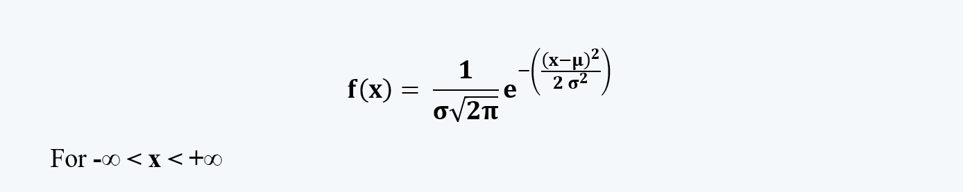
c. The probability density function of a normal distribution curve is:
d. Consider the following figure:
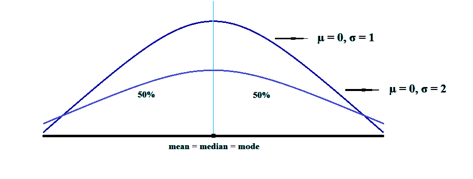
In the above figure:
i. The first curve, i.e. the higher one has a mean of 0 and a standard deviation of 1. It is called the standard normal distribution curve.
ii. The second one, i.e. the flatter one has a mean of 0 and a standard deviation of 2. The observations are more spread out in this curve. This curve, since it has a higher standard deviation, has a higher degree of volatility.
e. The approximate degree of concentration in a normal distribution curve is spread out as follows:
|
Spread |
Approx. Degree of Concentration |
|
µ ± 2/3 σ |
50% of observations |
|
µ ± σ |
68% of observations |
|
µ ± 2 σ |
95% of observations |
|
µ ± 3 σ |
99% of observations |
f. These are the approximate degrees of concentration of the probabilities, the more precise intervals are :
|
Confidence Levels |
Intervals |
|
90% |
x̄ ± 1.65s |
|
95% |
x̄ ± 1.96s |
|
99% |
x̄ ± 2.58s |
2.3. Standardizing a Random Variable
a. Z is the conventional symbol for measure for determining a standard normal random variable.
b. It can be calculated by subtracting the mean of X from X and then dividing the result by the standard deviation. It can be obtained by reducing the population mean from the observed value and dividing the result by the standard deviation.

c. If we have a sample instead, it can be calculated as follows:

d. For example, suppose we have the expected value of X as 15% and a standard deviation of 30%.
What will be the probability of X being less than or equal to 18%?
Here we have to find P(X ≤ 18%). To do the same we first find the value of Z as follows:

We can draw the same on a distribution curve as follows:
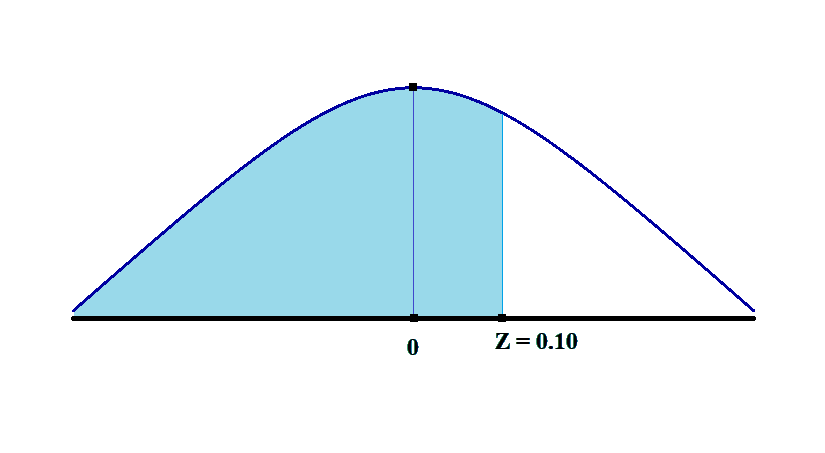
The probability of X being less than or equal to 18% is the shaded area under the curve to the right of the point Z = 0.10. We can find its value in the tables.
