LOS B to G requires us to:
b. describe the set of possible outcomes of a specified discrete random variable;
c. interpret a cumulative distribution function;
d. calculate and interpret probabilities for a random variable, given its cumulative distribution function;
e. define a discrete uniform random variable, a Bernoulli random variable, and a binomial random variable;
f. calculate and interpret probabilities given the discrete uniform and the binomial distribution functions;
g. construct a binomial tree to describe stock price movement
1. Discrete Uniform Distribution
a. The example discussed above is one of a discrete uniform function.
b. A discrete uniform distribution shows that the possibility of every finite possible outcome is equally likely.
c. For example, consider the following likelihood of the increase in the dividend distribution of a company:
|
Dividend Increase |
Probability |
Cumulative Probability |
|
0.05 |
0.2 |
0.2 |
|
0.1 |
0.2 |
0.4 |
|
0.15 |
0.2 |
0.6 |
|
0.2 |
0.2 |
0.8 |
|
0.25 |
0.2 |
1 |
|
Total |
1 |
In the above example:
i. The probability of an event, say an increase in dividends by 15 cents is 0.2 or 20%, i.e.:

ii. The probability of the increase is greater than 10 cents is 0.60 or 60%, i.e.:

d. Thus, we can deduce the following characteristics of a discrete uniform distribution:
i. The outcomes are countable,
ii. The probabilities of individual outcomes lie between 0 and 1

iii. The sum of all possibilities or probabilities is always 1

iv. The probability of any one of the outcomes for all possible outcomes is always 1/n, i.e.:

2. Binomial Distribution
a. A binomial random variable measures the number of successes in n trials.
b. A Bernoulli random variable has only two outcomes, i.e. 1 and 0. ‘1’ represents success, and ‘2’ represents failure.
Each of the outcomes is called a trial.
c. There may be a series of events, having two possible outcomes, i.e. success and failures. The total of successes out of the total number of observations being observed is called the binomial random variable. Thus,

d. For example, we are considering a stock’s price movements, and the prices may either move or down while transitioning from one period to another. Suppose, the outcomes of different trials and their values are as follows:
|
Trials |
T1 |
T2 |
T3 |
T4 |
T5 |
T6 |
T7 |
|
Outcomes |
U |
D |
D |
U |
U |
D |
U |
|
Values |
1 |
0 |
0 |
1 |
1 |
0 |
1 |
For the above data, the outcomes of prices going up are the ‘success’ outcomes. Thus the binomial random variable for the chances of stock prices going up would be (i.e. the number of ‘success’ outcomes divided by the number of total trials):

Now, let us suppose that the probability of the stock price going up is 60 % (such that p = 0.60), making the probability of stock price going down equal to 40% (i.e. 1-p = 0.40). We also observe that out of 7 trials, the total numbers of up-moves are 4 (i.e. x = 4) and the total numbers of down-moves are 3 (i.e. n-x = 3). The probability of a binomial random variable in the series would be:

e. We can generalize this equation to write a probability of the success of an event as:

This represents the probability of one particular way of getting success out of n trials.
f. Also, if the order of the event doesn’t matter, the probability of success amongst n trials is:

This also represents, the number of ways of getting x successes and (n-x) failures.
g. To find the probability of x successes given n trials, we need to multiply the above two equations.
Therefore,

2.1. Mean of the Binomial and Bernoulli Variables
a. Both binomial and Bernoulli variables are explained by two variables. The binomial variable is explained by n and p. And, the Bernoulli variable is explained by 1 and p.

b. The mean of the Bernoulli Variables can be calculated as follows:

c. The mean of the binomial variable, on the other hand, is:

2.2. Variance of Binomial and Bernoulli Variables
a. The variance of data can be calculated by using the following formula:

b. For the Bernoulli variables, the expected value or mean is ‘p’. Therefore, we can re-write the above equation of variance for the Bernoulli variables as follows:

Putting the expected value of the variables in the above equation, we get:

Solving this equation we get the variance of Bernoulli random variables as :

c. Similarly, the variance of Binomial trials is:

3. Binomial Applications
a. Suppose there is a series of events, like the price of stocks either moving up or down, such that:
i. The trials will take place thrice, one after another,
ii. The stock price going up is a success and going down is a failure,
iii. The probability of success is ‘p’; so that the probability of failure becomes ‘1-p’.
b. We have to find the number of successes and failures in the run of three trials, given that the order of success and failure doesn’t matter.
c. We can draw the binomial tree for the series as follows:
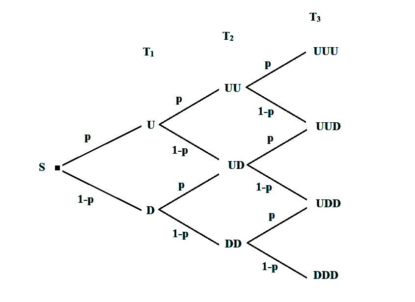
d. We can see from the above diagram that there are four possible outcomes, i.e. three up movements (UUU), two up and one down movement (UUD), one up and two down movements (UDD), and three down movements (DDD).
e. We can find the probabilities of each of the outcomes as follows:
i. The probabilities of the three up movements would be:

ii. The probability of two ups and a down is:

iii. Similarly, we can find the probabilities of other events and trials as well.
4. Tracking Errors
a. Tracking error is measured by the term Rp – Rb.
b. It measures how closely a portfolio follows its benchmark.
c. For example, suppose the expected tracking error for a stock’s prices should be 75 bps for 90% of the observations; such that, if for a trial Rp – Rb < 75 bps, it is considered as a success and if it is more than 75 bps, it is a failure.
If out of 8 trials observed, 6 witnessed the success; then what is the probability of viewing 6 or fewer successes in the observation of 8 trials.
We are therefore supposed to find . This can be calculated by finding the one minus the probability of x greater than 6. Thus,
