LOS A requires us to:
define a probability distribution and distinguish between discrete and continuous random variables and their probability functions
a. Probability distribution specifies the probabilities for the possible values of a random variable.
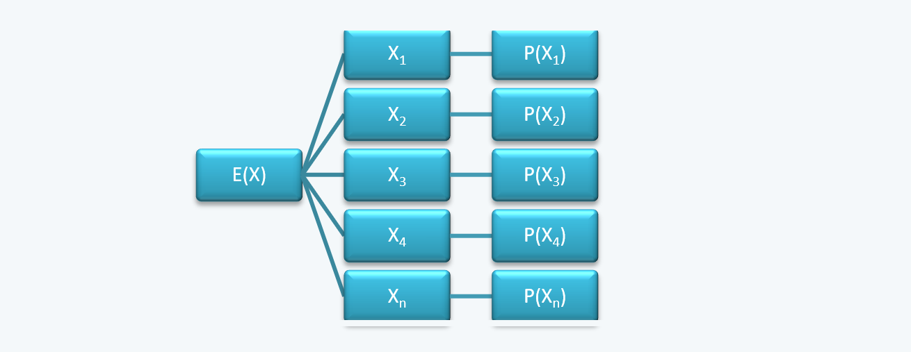
b. The probability function is the function of all the possible outcomes along with their associated probabilities. A probability function completely describes the variable, such that:
i. The probability of an individual variable lies between 0 and 1, i.e.

ii. And, the sum of probabilities of all variables is 1, i.e.

c. There are two types of random variables, i.e. discrete random variable and a continuous random variable.
1. Discrete Random Variable
a. A discrete random variable is a theoretically countable number of outcomes, such as:
i. A die has six sides, and we know the number of possible outcomes on rolling a die. We can also assign possibilities to each of these outcomes.
ii. The number of stars in the sky, which is ‘theoretically’ countable and not infinite, howsoever, large the number might be.
(The progress of the discrete numbers is in the sequence such as 1, 2, 3, and so on. It cannot be 1, 1.1, 1.2, etc.)
b. The function of a discrete random variable is the countable, non-zero probability for each outcome.
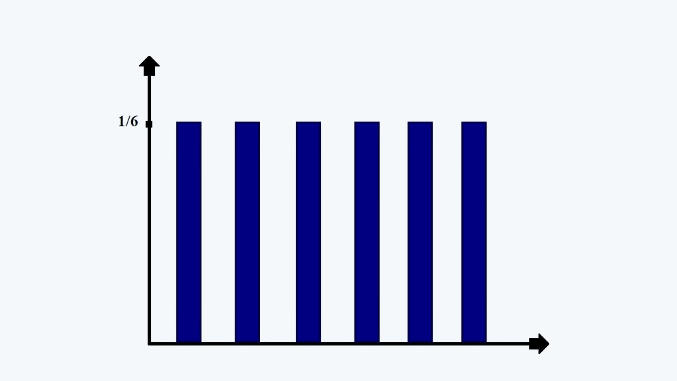
c. For example, the probability density function for a set of die rolled out can be written as:

or,

It can be depicted on a graph as follows:
d. Taking another example, suppose the expected dividends and their respective probabilities are as follows:
|
Dividends |
Probability P(x) |
|
0.05 |
0.05 |
|
0.1 |
0.25 |
|
0.15 |
0.45 |
|
0.2 |
0.15 |
|
0.25 |
0.07 |
|
0.3 |
0.03 |
|
Total |
1 |
This can be drawn on a graph as follows:
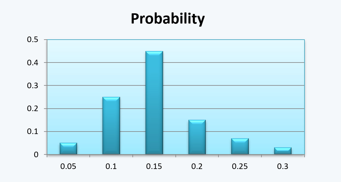
Here P(X=x) is the probability that ‘x’ takes on a specific value. For example, the probability of dividends being 15 cents is 0.45 or 45%.
We can also draw a cumulative distribution function graph for the same probability function as follows:
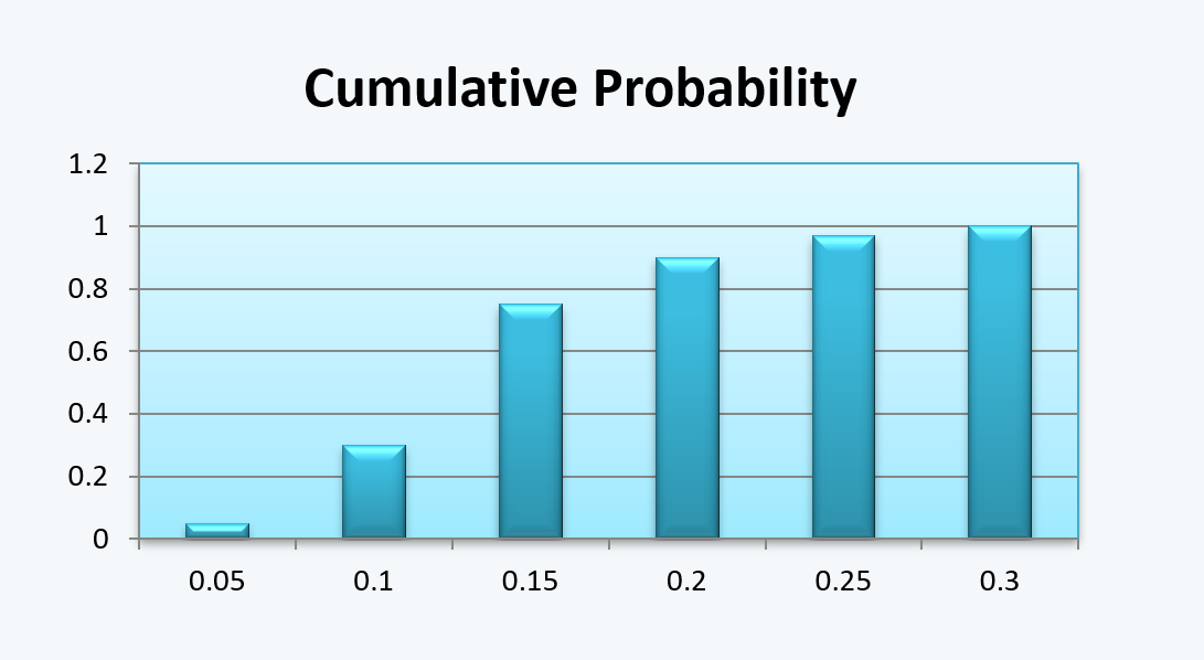
The cumulative distribution either remains the same or constant over each possible outcome.
Also, if we have to find the probabilities within a certain range of outcomes, it can be done as follows:
P(0.1 ≤ x ≤ 0.25) = 0.97 – 0.05 = 0.92 or 92%
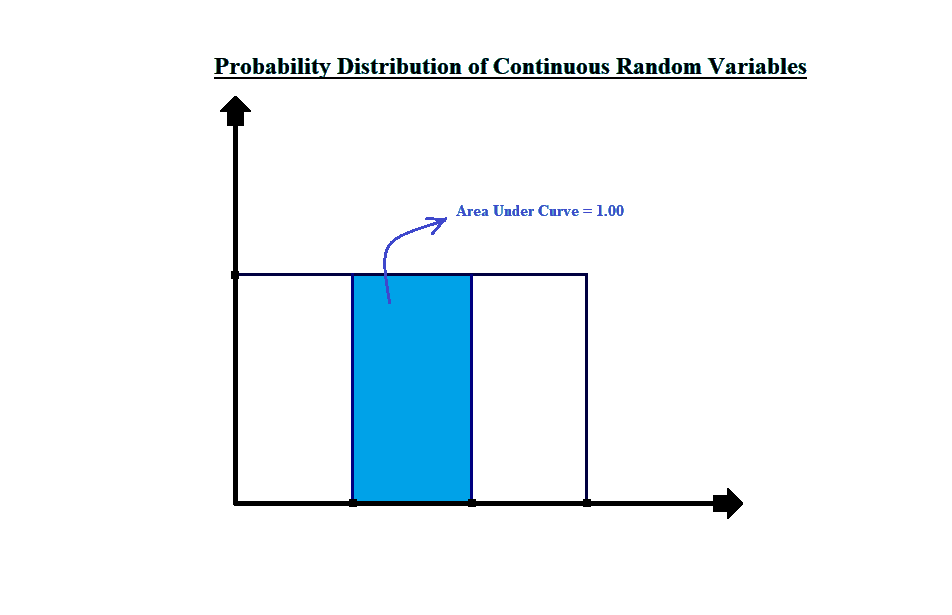
2. Continuous Random Variable
a. A continuous random variable series is not countable. For example, the return on the stocks (they have values in numbers such as 10.1%, 10.2%, 10.16%, etc.)
b. The function of a continuous random variable is the probability of each of the uncountable outcomes. It can be written as:
P (X = x) = 0
This is mainly because; there is an infinitely large number of outcomes, that the probability of individual outcomes is almost 0.
c. We plot the probability of the continuous variable by plotting the area under the curve and consider the data whose probabilities lie under a certain area. For calculating the same, the cumulative distribution is more important.
d. Consider the following example of a continuous-discrete function:
|
X=x |
p(x) = P(X=x) |
F(x) = P(X≤x) |
|
1 |
0.125 |
0.125 |
|
2 |
0.125 |
0.250 |
|
3 |
0.125 |
0.375 |
|
4 |
0.125 |
0.500 |
|
5 |
0.125 |
0.625 |
|
6 |
0.125 |
0.750 |
|
7 |
0.125 |
0.875 |
|
8 |
0.125 |
1.000 |
For the above distribution:
i. The probability of ‘x’ being less than 7 is the cumulative frequency of x up to 7, which is 0.875, i.e.

ii. The probability of ‘x’ having values between 4 and 6 are:

iii. And,
