LOS M requires us to:
calculate and interpret covariance given a joint probability function
a. The joint probability of two events is denoted by P(X, Y). It is the probability of X happening along with Y.
b. One thing that needs to be noted here is that we should not confuse this term with P(X|Y), which is the conditional probability of X, given that Y has already occurred.
c. For example, consider the following joint probability matrix:
|
Probabilities of Return on Assets |
RB |
|||
|
20% |
16% |
10% |
||
|
RA |
25% |
0.20 |
0 |
0 |
|
12% |
0 |
0.50 |
0 |
|
|
10% |
0 |
0 |
0.30 |
|
We can calculate the expected return on A and B by summing up the total probability of earning each level of returns and multiplying the same with their respective percentage returns. Thus, the expected return on asset A and asset B in the above matrix would be:

In slightly more complicated cases where the probabilities are even more distributed, like in the case of the probability matrix below:
|
Probabilities of Return on Assets |
RB |
|||
|
20% |
16% |
10% |
||
|
RA |
25% |
0.20 |
0.05 |
0.05 |
|
12% |
0 |
0.45 |
0 |
|
|
10% |
0 |
0 |
0.25 |
|
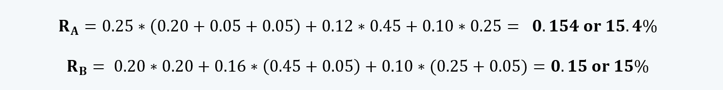
The expected return on both the assets would be:
d. We can also calculate the covariance of the joint probability function using the formula:

Thus for the initial matrix, where the expected return on A was 14% and the expected return on B was 15%, we can calculate the covariance as follows:
| RAi – E (RA) | RBj – E (RB) |
Cross Product |
P (RA RB) | COV (RA RB) | ||
|
(25-14)% |
=11.00% |
(20-15)% |
=5.00% |
55.00 |
0.2 |
11.00 |
|
(12-14)% |
= -2.00% |
(16-15)% |
=1.00% |
(2.00) |
0.5 |
(1.00) |
|
(10-14)% |
= -4.00% |
(10-15)% |
= -5.00% |
20.00 |
0.3 |
6.00 |
|
16.00 |
||||||
Hence the covariance between the return on assets A and B is 16%. Since this covariance is greater than 0, therefore the returns on these assets covary positively. This means that when the return on asset A is greater than the expected return on the asset then the return on Asset B is also greater than the expected return on asset A.