LOS G, H, and I require us to:
g. calculate and interpret the expected return of an asset using the CAPM;
h. describe and demonstrate applications of the CAPM and the SML;
i. calculate and interpret the Sharpe ratio, Treynor ratio, M2, and Jensen’s alpha.
1. Estimated Return on Securities
The expected returns on security can be calculated using the CAPM. This expected return can be used in valuing the securities, using the net present value (NPV) approach. There are basically three steps in this approach:
a. Estimate the E(Ri)
b. Calculate the expected annual cash flows using the probability of success.
c. Calculate the NPV.
Example:
Suppose there is a project with the following expected cash flows:
Year 1: Expected outflow of $ 500,000
Year 2: Expected outflow of $ 200,000
Year 3: A 50% probability of an outflow of $100,000 and a 50% probability of inflow of $ 500,000
Year 4: A 50% probability of $ 400,000 inflow
Year 5: A 50% probability of $ 400,000 inflow
Year 6: A 50% probability of $ 400,000 inflow and a 50% probability of inflow of $ 600,000
It is also known that the expected market return is 12% and the risk-free rate is 2%. The project has a beta of 2.3. We need to estimate the NPV of the project.
To calculate the NPV, we first need to calculate the estimated return on securities, as follows:

We would now calculate the expected cash flows and the NPV as follows:
|
Year |
Cash Flows |
PVF |
PVF |
PV |
|
1.00 |
(500,000.00) |
1/(1.25)1 |
0.8000 |
(400,000.00) |
|
2.00 |
(200,000.00) |
1/(1.25)2 |
0.6400 |
(128,000.00) |
|
3.00 |
200,000.00 |
1/(1.25)3 |
0.5120 |
102,400.00 |
|
4.00 |
200,000.00 |
1/(1.25)4 |
0.4096 |
81,920.00 |
|
5.00 |
200,000.00 |
1/(1.25)5 |
0.3277 |
65,536.00 |
|
6.00 |
500,000.00 |
1/(1.25)6 |
0.2621 |
131,072.00 |
|
NPV |
(147,072.00) |
Since the NPV of the project is negative, it should be rejected.
2. Portfolio Performance Evaluation
There are many measures of portfolio performance. Some of them are:
2.1. Sharpe Ratio
This ratio calculates the average return earned in excess of the risk-free rate, per unit of volatility. It is calculated as follows:

This ratio measures the returns per unit of both systematic and non-systematic risk.
2.2. Treynor Ratio
This ratio calculates the average return earned in excess of the risk-free rate, per unit of diversifiable risk. It is calculated as follows:

2.3. M-Squared (M2)
This ratio was created by Franco Modigliani and his granddaughter, hence named M2. This ratio is an extension of the Sharpe Ratio. It gives us the excess return on the portfolio adjusted for the market risk minus the excess return on the market. This ratio also considers the total risk. M2 can be calculated as follows:

2.4. Jensen’s Alpha
This ratio gives us the difference between the actual and the expected return. This ratio is calculated as follows:

3. Security Selection
So far in all the models discussed above, we have assumed that there is homogeneity in the investors’ expectations. But here in this section, we introduce the heterogeneity in expectation of the investors. But, since the investors are the price takers, this heterogeneity does not affect the markets much.
The differences in the expectations of investors could be on the account of differences in the beliefs with respect to:
i. future cash flows,
ii. systematic risk of the security, or
iii. both
We can make the security selection based on Jenson’s Alpha, which, based on the past results, shows indicates the superior and inferior securities.
Another way of making the security selection is through plotting the SML, as follows:
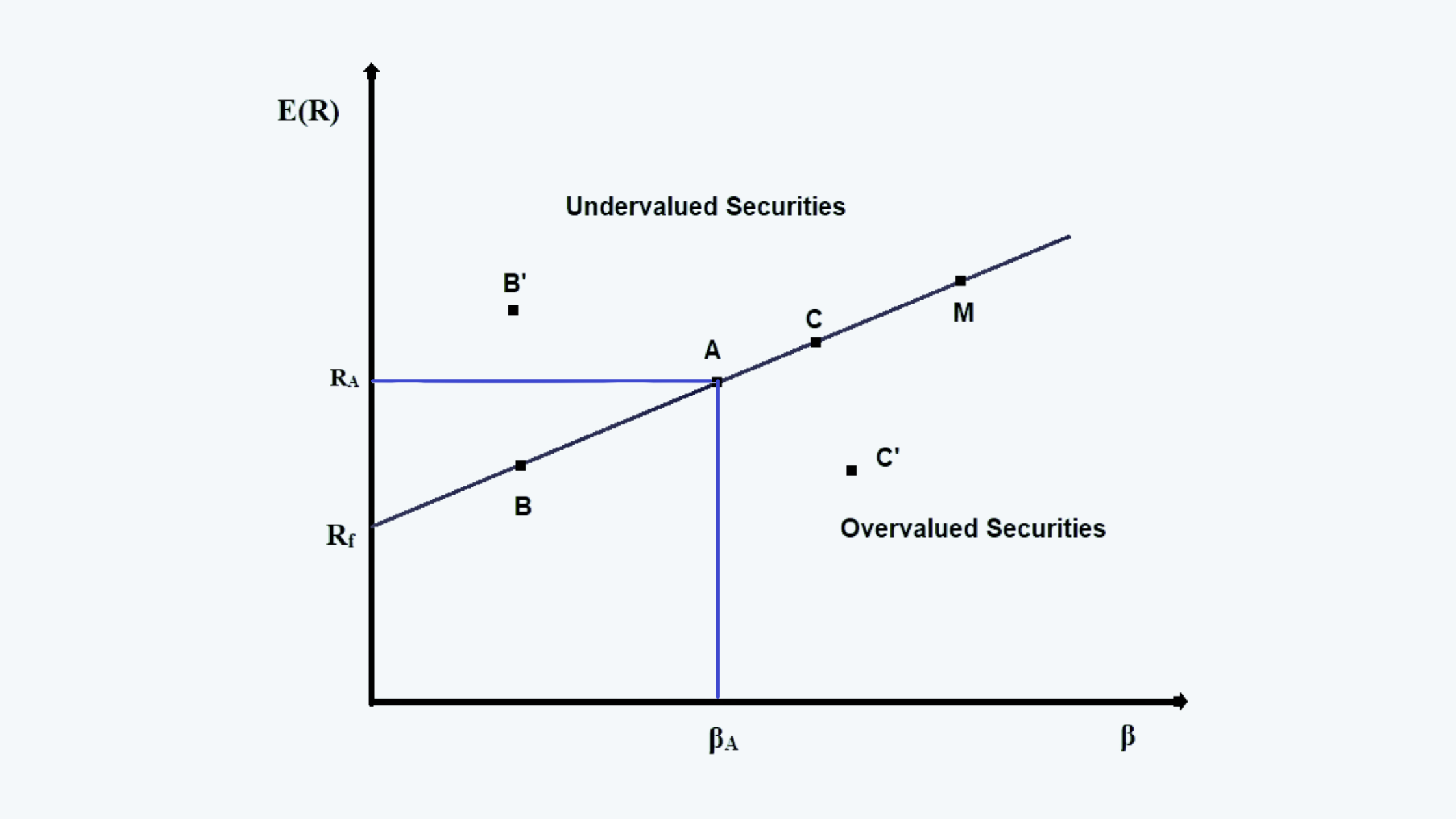
In the above figure, all the points on the SML represent the market expectations or the consensus view of the security’s return. All the points above or below the line are individual expectations. The points above the SML, such as B’ have higher expected returns, as perceived by the individual. Thus, it represents the undervalued security. Similarly, all the points below the SML represent the overvalued securities.
Obviously, while making the selection the undervalued securities should be purchased.
4. Security Characteristic Line
This line is constructed using Jensen’s alpha. The equation for Jensen’s alpha is:
We can rearrange the terms of this equation as:

In the above equation:
i. (Ri – rf) is the dependent variable and represent an excess return on i, and
ii. (Rm – rf) is the independent variable and represents an excess return on market.
This can be presented graphically as follows:
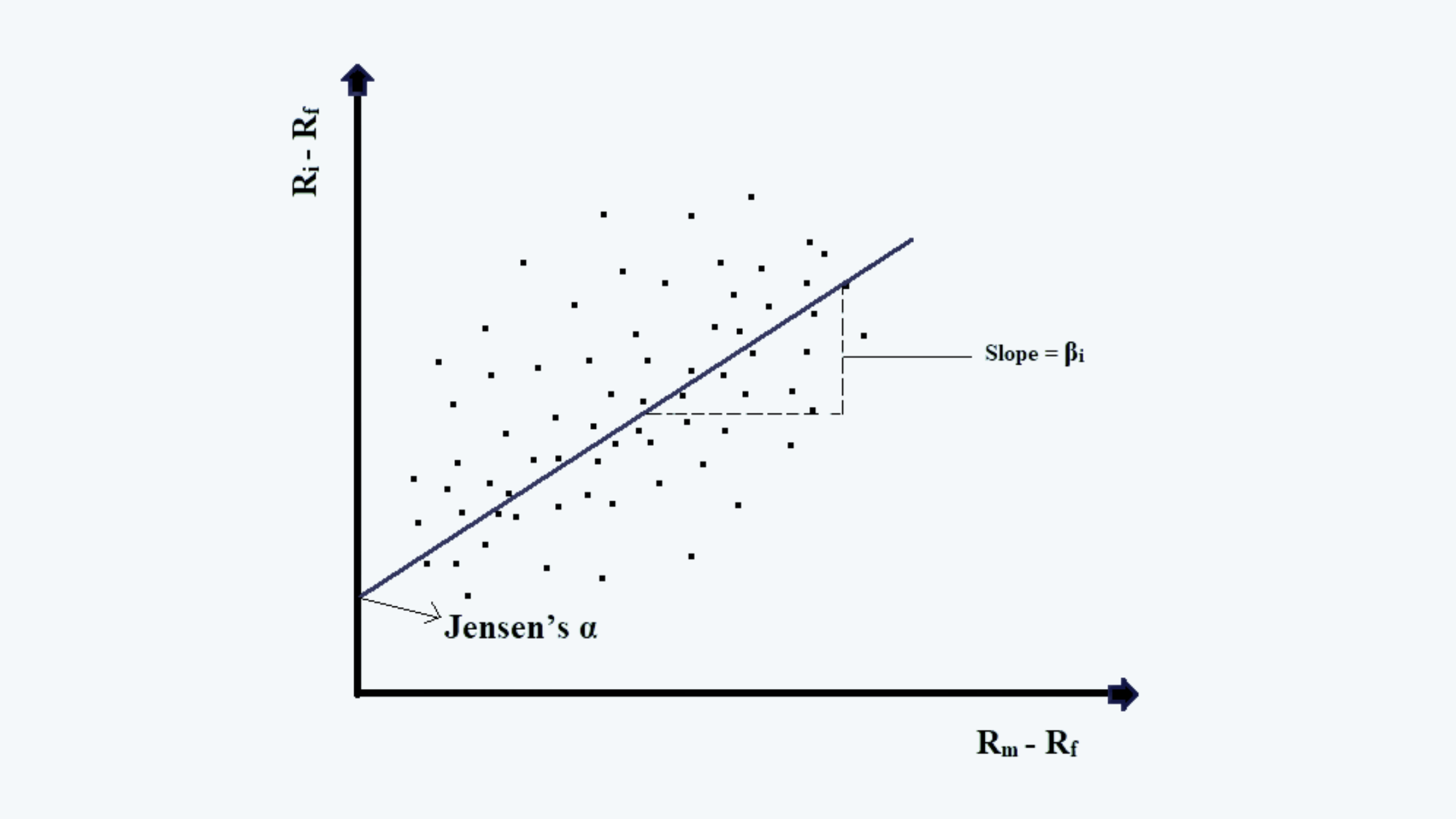
In the above figure, the slope of the line is β and the intercept is α.
The selection of the securities should be made as follows:
i. select the overweight securities whose alpha is greater than zero, and
ii. deselect the underweight securities whose alpha is less than zero.