LOS D requires us to:
explain return generating models (including the market model) and their uses
As per what we have discussed so far:
a. the non-systematic risk can be avoided, and therefore it is no rewarded;
b. the securities are priced to reward systematic risks only; and
c. securities with more systematic risk should offer a higher return.
Constructing an Optimal Portfolio
a. If we were to construct the market portfolio, we would have to consider all the available assets that are investible and tradable.
b. So for ease, let us consider an index with 1000 assets of it, as our market portfolio, we would be required to determine the return on our portfolio and variance on it. This would basically require 1000 return estimates, 1000 estimates for standard deviation, and 499,500 (i.e. 1000*999/ 2) correlation coefficients.
c. So, as an alternative we can begin with a known portfolio, i.e. an equity index such as S&P 500:
i. We can measure its expected return (E(Rm)) and its risk (σ2) using the historical data. (The variance of market portfolio acts as the benchmark for systematic risk).
ii. We then compare the returns on the securities (Ri) with the market return (Rm) using a linear regression model.
iii. The security’s systematic risk can be calculated using the following formula:

So, if the investor gets rewarded for the systematic risk only, this way we can determine what the expected would be.
Multi-Factor Model
a. It is a model that can help in providing an estimate of the expected return on a security.
b. A multi-factor model, based on past data, identifies the major factors that impact the risk and return of a security. Such factors could be macroeconomic (such as growth, interest rates, etc.), fundamental factors (such as earnings, cash flows, etc.), statistical factors, etc.
c. We can develop a model, that gives us the expected return, as follows:
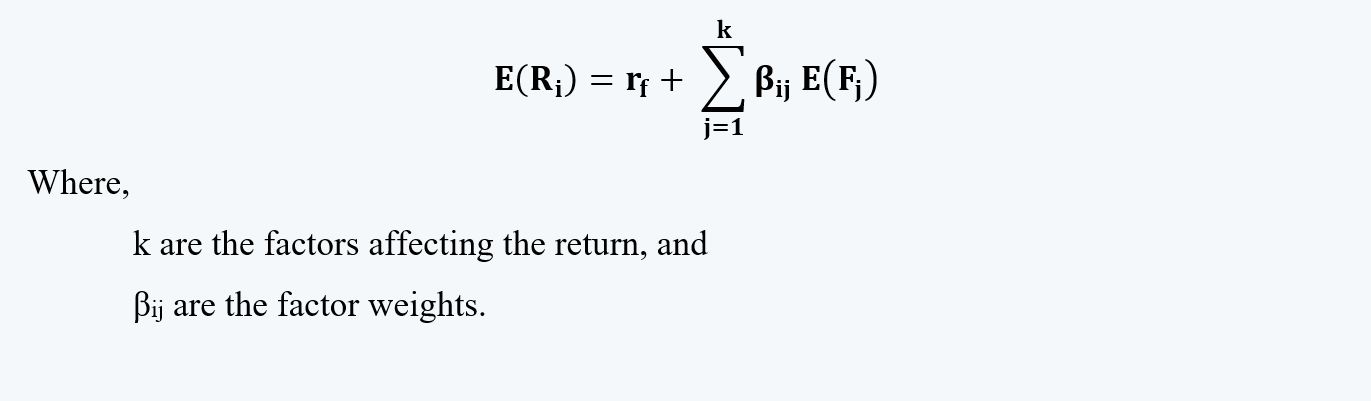
d. We can write the above equation as
e. We can add one more factor that does impact the return on a security, i.e. the excess market return. After the inclusion of this factor, the model would look like this:

In regression, the inclusion of [E(Rm) – rf] will absorb the variance from other factors.
Single-Factor Model
a. In the previous model, we had multiple factors that affected the returns on security, to start with. Then, we’d put the first factor that most importantly affected the return on the securities, i.e. excess market return.
b. So when we put the market return as a factor, the other factors are not that important anymore. So, in order to keep the model simple, we drop out the other factors that affect the return.
c. So, a single-factor return generating model would look like this:
E(Ri) – rf = ꞵi [E(Rm) – rf]
This is also the equation for the Capital asset Pricing Model or CAPM.
d. We can also write this linear equation in terms of expected return as a function of market return and a risk-free rate:
E(Ri) = rf + ꞵi [E(Rm) – rf]
e. We have seen the equation of the capital market line above, which is:

In the above equation, if we replace the Rp with Ri, because here our asset only constitutes the portfolio. And rearrange the equation, as follows:

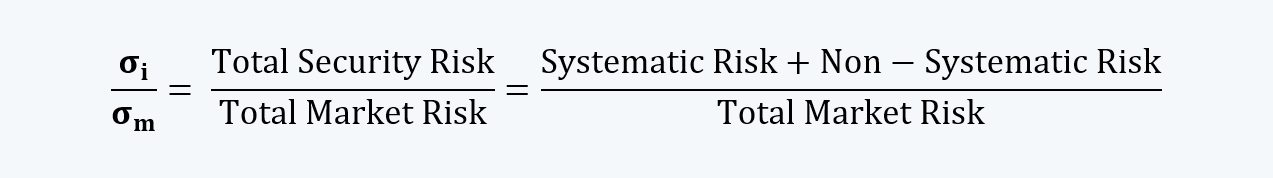
If we compare this equation with the first equation of the single-index model, we can infer that:

Therefore, a beta of a security is nothing but the total security risk divided by the total market risk.
f. Now, the total security risk is made up of two components, i.e. systematic and non-systematic risk. Thus:
But, we have learned above that investors don’t get rewarded for the non-systematic risk. Thus,

But, we know that security systematic risk is some function of beta and total market risk. Therefore:

This is the other way of proving that the single-index return generating model is consistent with the CML model.
g. Now that we have got the equation for the single-index model, which is:
We can rearrange this equation as follows:

We can rearrange this equation as follows:

Now, we move from the expected to the actual values, and term rf (1 – ꞵ) as α. The equation for the market model would thus be:
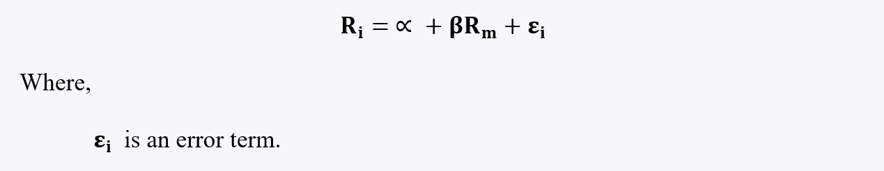
α and β can be estimated using the historical security market returns.
Example:
Suppose there is a security, A, and an index M, whose historical data shows an α of 0.0001 and β of 0.9.
Therefore the equation of the single index model of the security would be:
RA = 0.0001 + 0.09 Rm + ɛA
Now, if during a particular day the return on the security and the index were 1% and 2% respectively. Then the return on security due to the non-systematic risk would be:
=0.02 – (α + βRm) = 0.02 – (0.0001+ 0.9*0.01)
= 0.0109 or 1.09%.